Melbourne SCATS Traffic Analysis 2014–2026:
Congestion, Volume, Interactive Maps and OOH Billboard Intelligence
A unified, deduplicated and cleaned Melbourne SCATS traffic intelligence platform covering
539+ billion cleaned vehicle movements,
12+ years of history,
15-minute behavioural analytics,
interactive maps, suburb commute intelligence, OOH opportunity discovery, database diagnostics,
data-quality evidence and reproducible open-source workflows.
Melbourne Traffic Data, Congestion Hotspots and Billboard Exposure Intelligence
This page brings together
Department of Transport Melbourne SCATS traffic signal data
,
cleaned traffic-volume outputs, interactive maps,
busiest-site rankings, congestion findings,
yearly and daily movement intelligence,
database diagnostics and OOH billboard exposure intelligence.
The Melbourne SCATS Intelligence platform is fully reproducible,
with analytical workflows, processing scripts, diagnostics,
data-quality systems and supporting methodology being released
publicly through the GitHub repository.
Found this platform useful?
Please consider sharing the Melbourne SCATS Intelligence Platform with
journalists, transport planners, engineers, developers,
OOH media professionals, freight/logistics observers,
researchers or anyone interested in Melbourne traffic intelligence.
539+ billion cleaned vehicle movements,
12+ years of Melbourne traffic intelligence,
interactive maps, diagnostics, data-quality evidence and
a reproducible open-source analytical workflow.
Popular Melbourne Traffic and OOH Opportunity Maps — Quick Access
These are likely to be the most-used parts of the page, so they now sit near the top for immediate access.
New council-level traffic intelligence section:
The Melbourne SCATS platform now includes a dedicated council traffic intelligence index covering all 31 council areas in the Greater Melbourne traffic report set. This section links directly to the council report index, where each council can be opened as an individual public traffic evidence page.
This council layer is designed for fast public understanding. Residents, councillors, MPs, council candidates, journalists, community groups and transport observers can start with a familiar boundary — the local council — and then inspect the traffic evidence for that area.
Council Areas
31
Evidence Types
SCATS + TIRTL
Report Format
HTML Index
Public Access
Open
Why the council reports matter:
Councils are the easiest civic boundary for most people to understand. The council reports turn public transport datasets into public traffic intelligence: visible, searchable, comparable and easier to share than internal GIS layers or one-off consultant reports.
The reports are not intended to replace council systems. They provide a public evidence layer built from open transport data, allowing traffic pressure, busy sites, freight signals and council-level patterns to be inspected from one public entry point.
Executive summary — 17th May 2026:
This platform represents one of the largest independently processed open SCATS analytical environments publicly assembled in Australia. It converts more than 12 years of Melbourne traffic signal data into a reproducible transport intelligence platform covering cleaned 15-minute observations, yearly and monthly movement history, site rankings, corridor behaviour, OOH parcel opportunity discovery, cinematic movement visualisations, database diagnostics and data-quality evidence.
This is no longer simply a statistics page. It is a public analytical infrastructure layer for journalists, OOH media, freight/logistics observers, researchers, government readers, developers and the general public. The platform combines historical SCATS intelligence with an expanding TIRTL pathway for freeway speed, vehicle class, heavy-vehicle and corridor-performance analysis.
Unlike conventional dashboard-style summaries, this platform exposes the analytical process itself: structural diagnostics, database inventory, month-coverage auditing, duplicate-key evidence, interval-quality checks, processing-time transparency, downloadable CSV/JSON outputs and reproducible scripts.
Cleaned Observations
37.877B
Cleaned Movements
539.021B
Detector-Day Rows Audited
401.123M
Database Footprint
97.95GB
Coverage Window
2014–2026
Month Audit
148 expected / 0 unexplained missing
Duplicate Key Audit
0 duplicate detector-day keys
Time Resolution
15-minute intervals
Why this matters:
The public charts show Melbourne’s movement story; the diagnostics prove the machinery behind it. The project demonstrates that open government transport datasets, DuckDB, HPC-style chunked processing, reproducible scripts and independent infrastructure can produce city-scale transport intelligence previously associated with institutional environments.
The strongest current capability is historical SCATS intelligence: yearly totals, daily and monthly trends, time-of-day behaviour, weekday/weekend patterns, day-of-week and seasonal profiles, busiest-site rankings, site-month intelligence, OOH exposure analysis and interactive mapping. The next major expansion path is deeper SCATS + TIRTL integration for freight, freeway speed, vehicle class and corridor-performance intelligence.
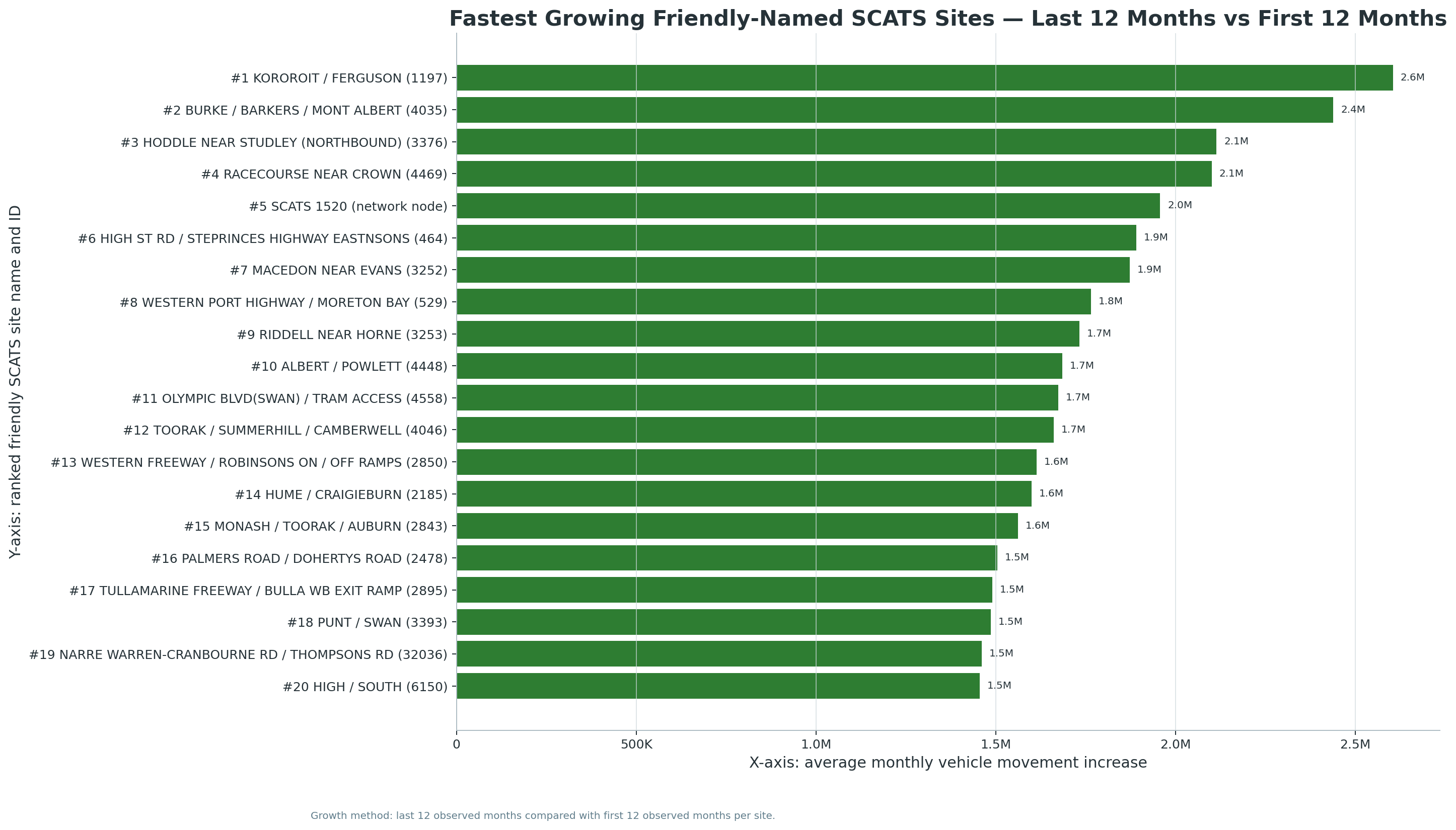
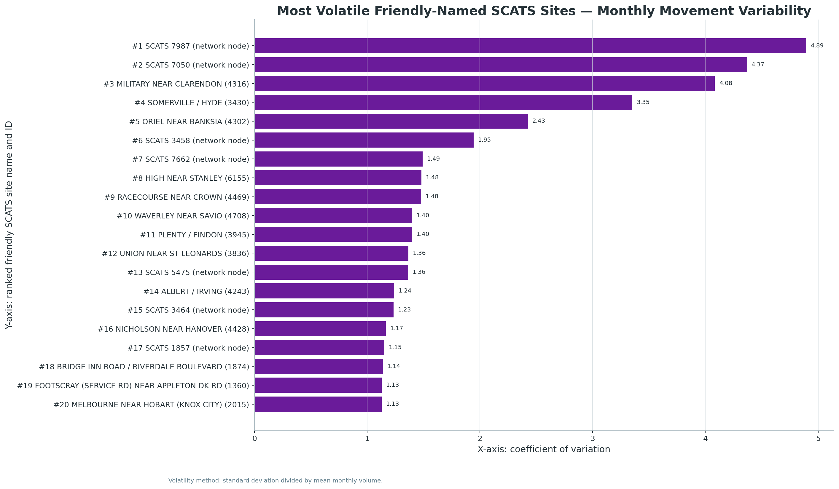
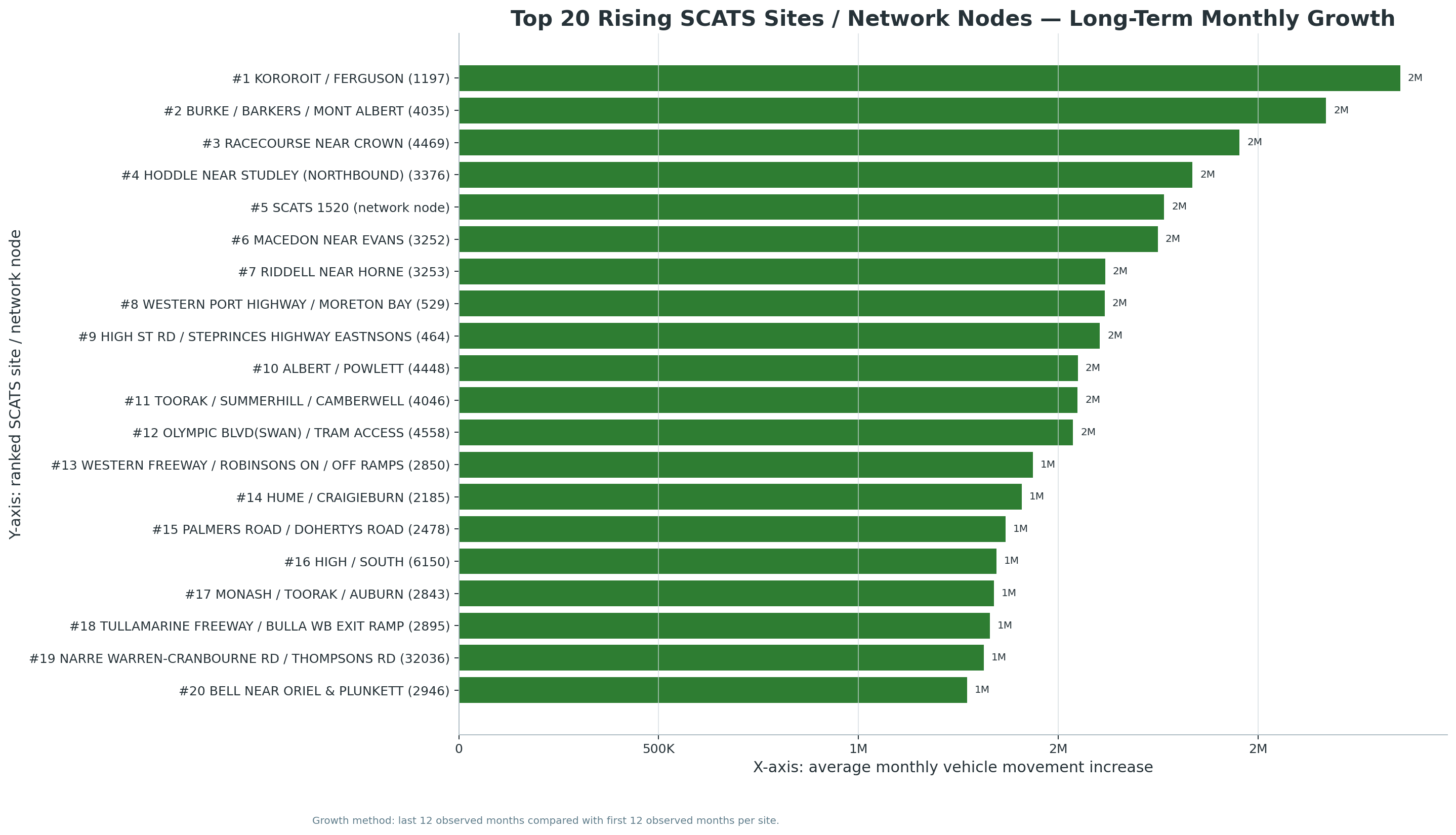
New V5.2 site-month download set:
The following chart and CSV outputs support the new Site-Month Traffic Intelligence module, including named SCATS sites, network-node labels, fastest growth, volatility, seasonality, and top-site trends.
Updated with busiest-site, busiest-day, busiest-time, quietest-time, peak-share, and V3 headline-merge findings
Database Footprint
102.7 GB on disk
Ranked Site Intelligence Sites
4,758
Top 1000 Portfolio Share
46.3%
Top 2000 Portfolio Share
71.9%
Sites Needed for 90% Traffic
~3,080
🧭 Explore the Melbourne SCATS Intelligence Platform
A guided index for journalists, transport planners, advertisers, researchers, councils, developers and the public.
The page now follows a deliberate reading path: scale → latest updates → findings → maps → local intelligence → behavioural analytics → commercial value → media value → proof → technical appendix.
1. Start Here — Executive Summary & Key Findings
Understand the scale, headline numbers and why the work matters before going deeper.
This section tracks new Department of Transport and Planning SCATS and TIRTL open-data releases as they become available.
The purpose is simple: turn raw open-data releases into rapid, readable traffic and freight intelligence.
When new SCATS or TIRTL data is released, the update can be processed into headline movement totals, busiest SCATS signal locations, strongest SCATS movement increases, highest-volume TIRTL truck locations, truck-share hotspot tables, mapped report locations, anomaly and watchlist candidates, publication caveats, method notes and supporting CSV evidence.
Latest brief — Melbourne Traffic & Freight Intelligence Brief, June 2026 Open Data Update
This automated brief covers the newest data window not included in the earlier SCATS and TIRTL project outputs.
SCATS Window
8 Apr – 11 Jun 2026
TIRTL Window
23 May – 11 Jun 2026
SCATS Movements
9.15B
SCATS Sites
4,612
TIRTL Vehicles
326.2M
TIRTL Trucks
48.1M
What each monthly brief tracks
busiest SCATS signal sites;
strongest SCATS movement increases;
heaviest TIRTL truck locations;
highest truck-share hotspots;
SCATS and TIRTL anomaly / watchlist candidates;
map panels and clickable report locations; and
supporting CSVs, named tables, maps and methodology notes.
Why this matters
DTP open data is valuable, but raw data releases are difficult for most people to interpret. This reporting pipeline turns each release into a concise traffic and freight intelligence briefing with named sites, ranked tables, map panels and supporting evidence.
The important point is not only the individual report. It is now a repeatable monthly capability: from open data release to media-ready traffic intelligence in under 30 minutes once the data is available.
Responsible-use note: Watchlist and anomaly rows are useful story leads for review, but they should not be treated as automatic proof of cause. Public claims should check named locations, road-name text, map coordinates and any unusual movement changes before publication.
The monthly brief archive is designed to grow as new DTP SCATS and TIRTL releases are processed. The stable latest links can be updated each month while the dated release folders preserve the historical archive.
The completed V3 headline merge, monthly totals, daily totals, site-intelligence, time-bin, and peak-share workflows now provide enough confirmed data to support three public-facing Top 10 sections. These findings are designed for fast reading by journalists, public readers, transport analysts, government agencies, researchers, and out-of-home media planners.
Why this section matters: the page has moved from a technical database demonstration into a publishable Melbourne traffic intelligence briefing. It can now tell readers how much Melbourne moved, when it moved, where the heaviest signalised load was concentrated, and why the network behaves the way it does.
Top 10 Network Findings — What Melbourne Actually Does
These are the broadest confirmed findings from the unified SCATS archive. They explain the true scale of the dataset and the actual movement patterns visible across Melbourne's signalised road network.
1Melbourne generated more than 539 billion vehicle movements
The completed total-cleaned-volume process confirms 539,020,710,239 cleaned vehicle movements across 148 / 148 months.
The unified cleaned archive contains 37,877,397,311 usable 15-minute observations.
3The system covers 4,907 SCATS sites
The archive confirms 4,907 distinct SCATS sites across the original, continuation, and recovery databases.
4The loaded archive spans more than 12 years
The unified date range runs from 2014-01-01 to 2026-04-07, giving the page long-run historical context.
5October 2025 was the highest-volume month
The completed monthly totals process identifies 2025-10 as the highest-volume month, with 4,513,402,918 cleaned vehicle movements.
6Friday 12 December 2025 was the busiest recorded day
The completed daily totals process identifies Friday 12 December 2025 as the busiest recorded day, with 166,208,622 cleaned movements.
7PRINCES NR CANNING is the busiest confirmed site
SCATS site 4415 — PRINCES NR CANNING is currently the busiest ranked site, with 674,498,771 total cleaned vehicle movements.
8The page has a complete daily record layer
The completed daily totals workflow confirms 4,437 daily records, enabling day-by-day comparisons and event discovery.
9The three DuckDB archives occupy about 102.7 GB
The SCATS analytical databases occupy approximately 102.7 GB on disk, explaining why chunked workflows were required.
10The V3 headline merge is complete
The final headline merge confirms all required sources are present and complete: total volume, busiest site, busiest day, busiest time bin, and peak shares.
Top 10 Congestion Findings — Where and When Pressure Builds
These findings explain the time-of-day and concentration patterns that define Melbourne's pressure points.
1Almost 40% of all traffic occurs in six peak hours
The combined AM and PM peak windows account for 37.45% of all cleaned vehicle movements.
2The afternoon peak is stronger than the morning peak
The PM peak accounts for 20.54% of all movements, compared with 16.91% for the AM peak.
317:15 is Melbourne's busiest 15-minute traffic interval
The busiest network-wide time bin is 17:15, averaging 2,283,898 movements per day across 4,437 dates.
403:00 is the quietest network interval
The quietest average daily time bin is 03:00, averaging 151,358 movements per day.
5The PM peak alone represents more than 110 billion movements
The afternoon peak window from 16:00–19:00 contains 110,696,055,470 cleaned vehicle movements.
6The AM peak alone represents more than 91 billion movements
The morning peak window from 07:00–10:00 contains 91,161,505,910 cleaned vehicle movements.
7Traffic load is highly concentrated
The top 100 ranked sites account for 7.8% of ranked traffic, while the top 500 account for 28.0%.
8The top 1,000 sites carry nearly half the ranked traffic
The top 1,000 sites account for 46.3% of total ranked traffic.
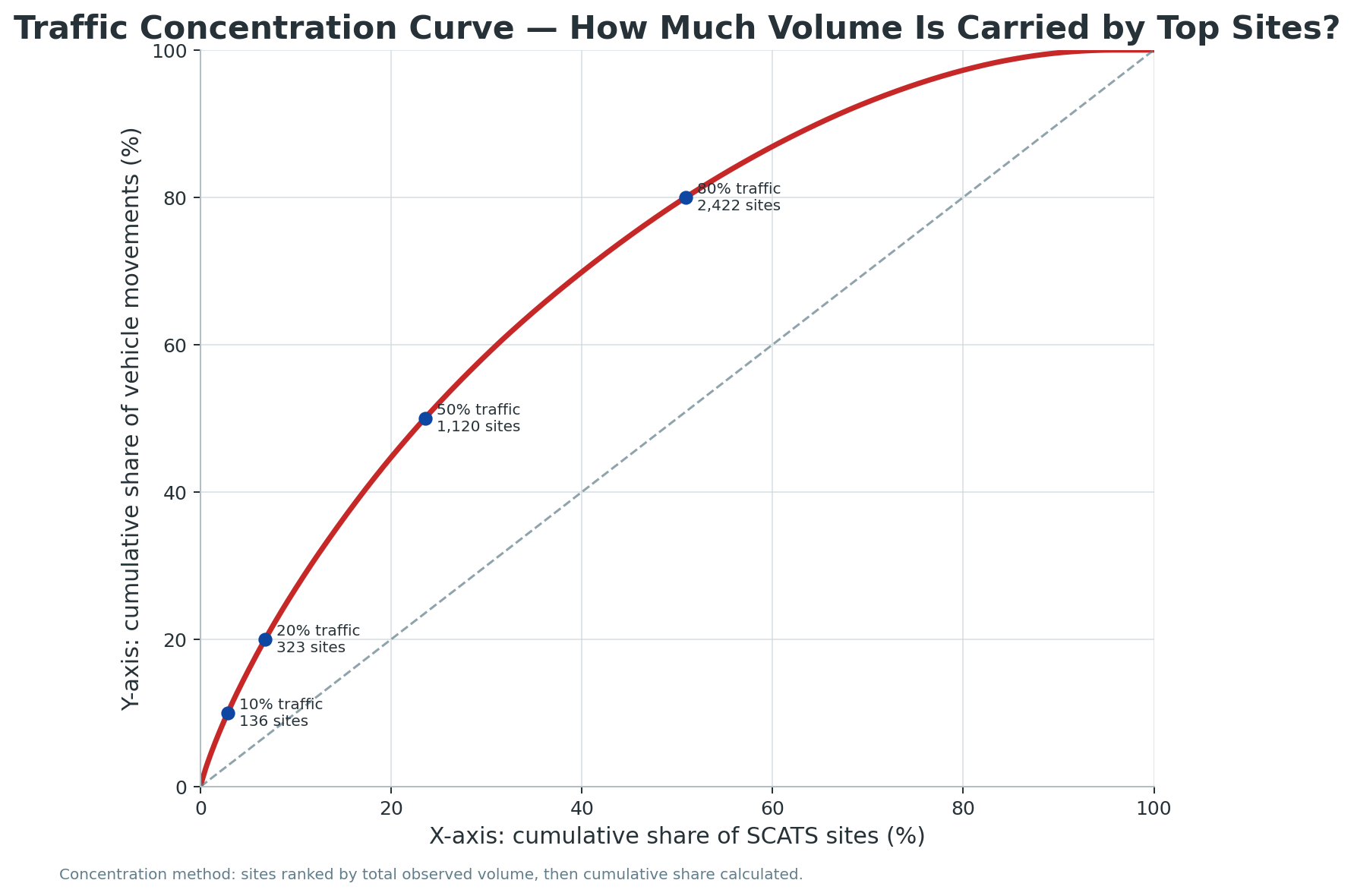
9About 1,120 sites carry half the traffic
The threshold analysis shows approximately 1,120 sites are required to capture 50% of ranked traffic.
10About 3,080 sites capture 90% of ranked traffic
The threshold analysis shows approximately 3,080 sites are required to capture 90% of ranked traffic.
Top 10 Strategic Infrastructure Insights — What Matters Long-Term
These findings translate the technical outputs into strategic value for government, media, researchers, advertisers, and infrastructure decision-makers.
1Melbourne's traffic backbone is measurable
The concentration analysis shows that a minority of sites carry a disproportionate share of traffic, making the city's practical movement backbone identifiable.
2The archive can support evidence-based corridor prioritisation
Site rankings, monthly volumes, daily totals, and time-bin profiles can help identify where infrastructure attention would have the greatest network effect.
3Peak-period policy can be tested against hard numbers
With 37.45% of traffic occurring in six peak hours, congestion policy can be assessed against quantified demand windows.
4OOH media planning can be ranked by actual movement load
The site-intelligence and portfolio-efficiency layers can help identify high-exposure traffic locations instead of relying only on broad assumptions.
5The system can generate journalist-ready public interest stories
The page now has named places, dates, totals, peaks, and trend layers that are understandable to the public and useful for news media.
6Monthly and daily trends allow disruption detection
Completed monthly and daily totals create a foundation for identifying COVID effects, seasonal surges, public-event spikes, and network disruptions.
7The system proves citizen-scale infrastructure analytics is possible
A privately built pipeline has processed a city-scale traffic archive using on-site computing, chunked analysis, and reproducible output files.
8The SCATS + TIRTL combination can move beyond intersection counts
SCATS provides signalised intersection volumes, while TIRTL can add freeway-grade speed, classification, and corridor behaviour.
9The platform can become a public traffic transparency layer
By publishing outputs, charts, methods, and downloads, the page can become an independent reference point for Melbourne movement analysis.
10The next breakthrough is interactive and predictive intelligence
The current foundation supports future live overlays, historical playback, incident comparison, corridor animations, predictive models, and natural-language querying.
Suggested reader takeaway: this is no longer just a statistics page. It is becoming an independent Melbourne traffic intelligence platform.
This work gives Melbourne a rare independent view of its signalised traffic network across more than a decade. It helps explain congestion, recovery, behavioural change, commuter rhythm, seasonal pressure, commercial exposure, freight context and public infrastructure questions in a form journalists, executives and residents can inspect.
The public value is not just the charts. It is the combination of cleaned data, reproducible compute, interactive maps, visual storytelling, OOH/parcel intelligence and a question-to-answer index that turns raw traffic counts into a practical city movement intelligence platform.
Yearly Totals Intelligence — Melbourne's Macro Traffic History
Yearly totals completed — 12 May 2026:
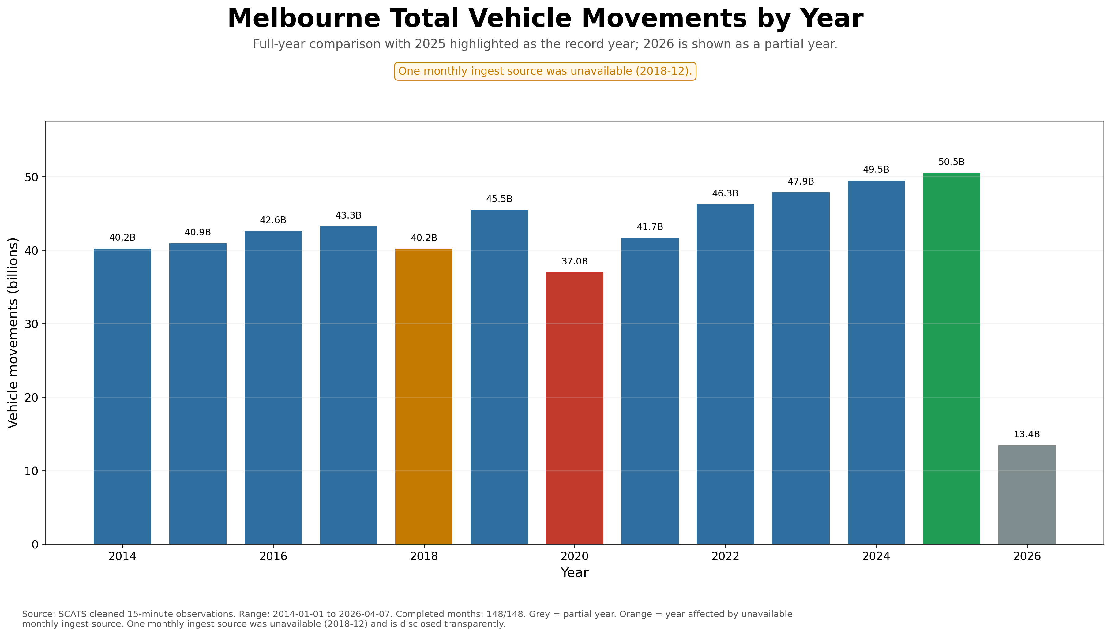
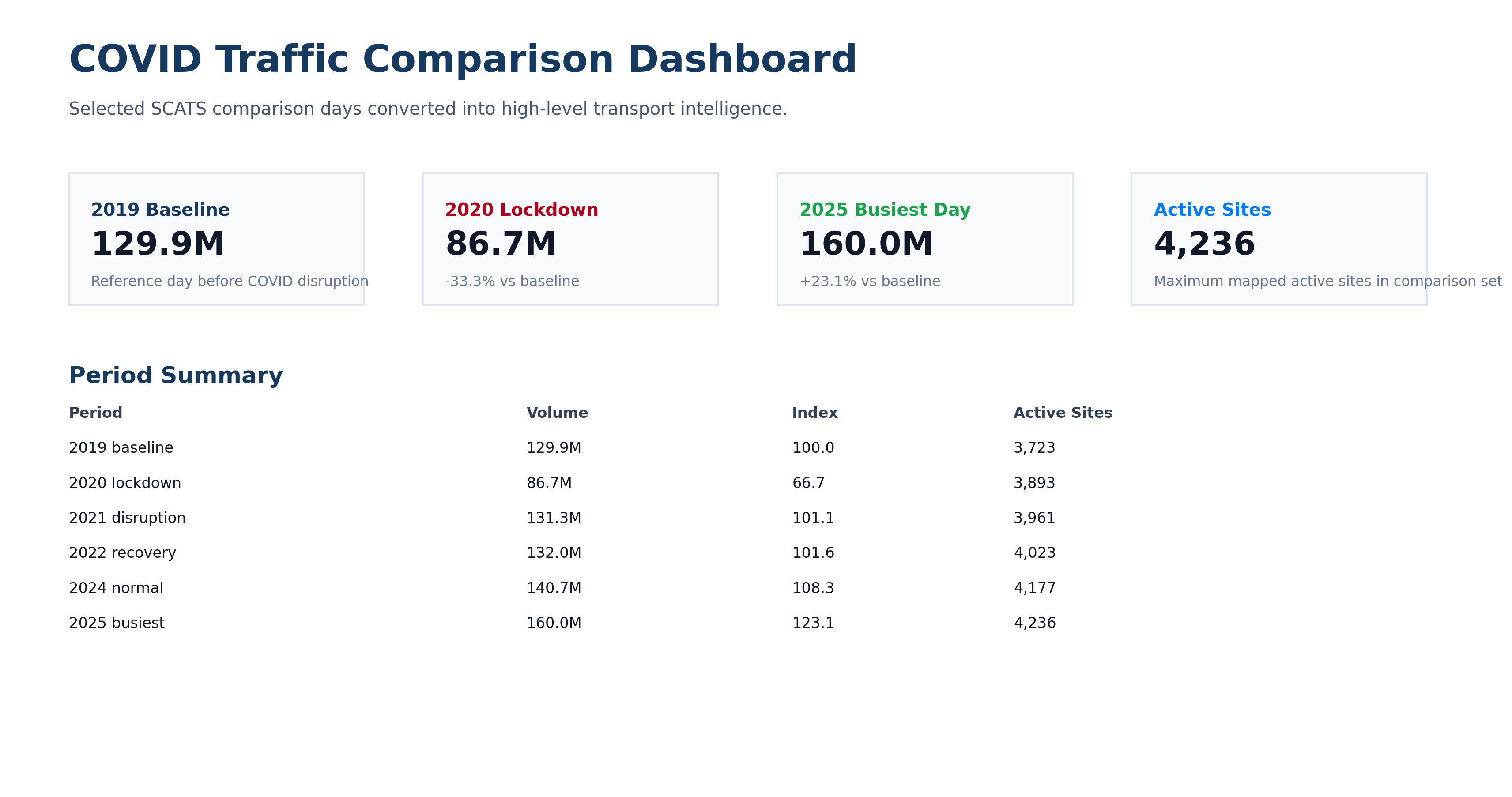
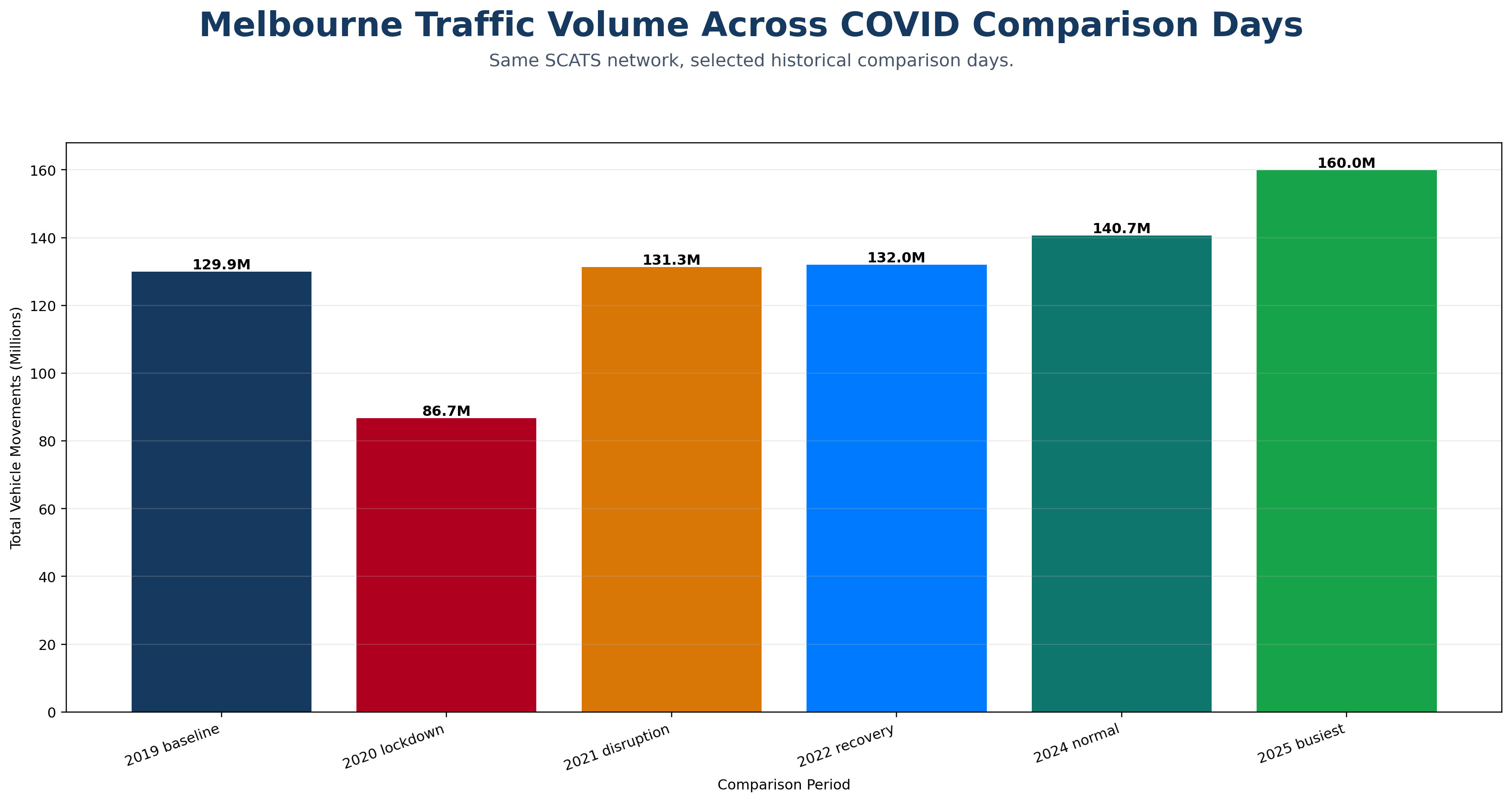
The yearly totals workflow is now complete across the full SCATS analysis window from 2014-01-01 to 2026-04-07, with 148/148 months processed. This gives the page a clean macro layer: long-term growth, the COVID-period collapse, the recovery phase, the 2025 record year, and the partial 2026 continuation period.
The yearly totals are one of the most important public-facing parts of the platform because they compress the entire 15-minute SCATS processing pipeline into a simple historical story. Viewers can immediately see Melbourne's traffic growth, the 2020 shock, and the post-COVID recovery into a new record year.
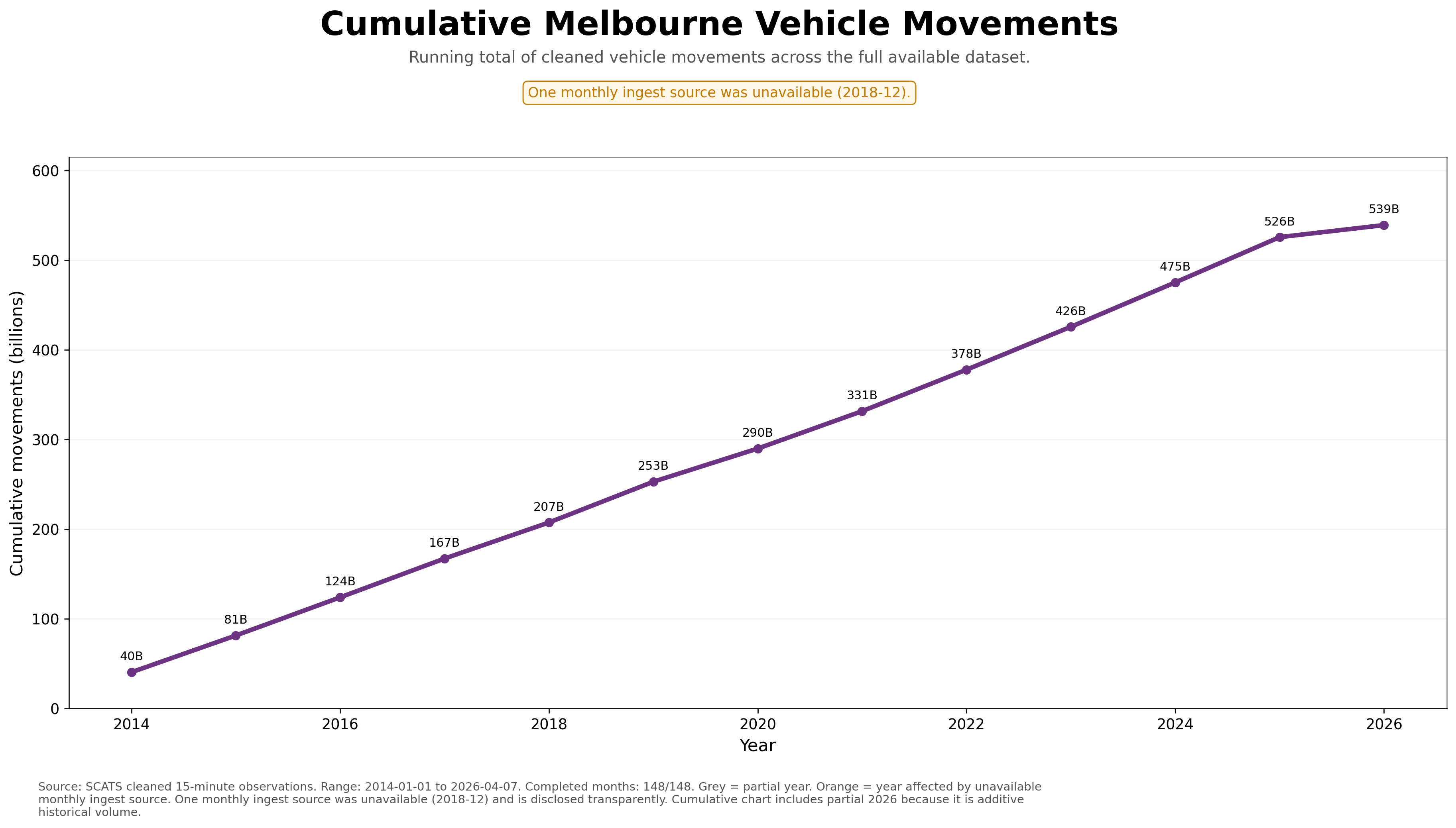
Cumulative movements
539B+
Running cumulative total across the available 2014–2026 dataset.
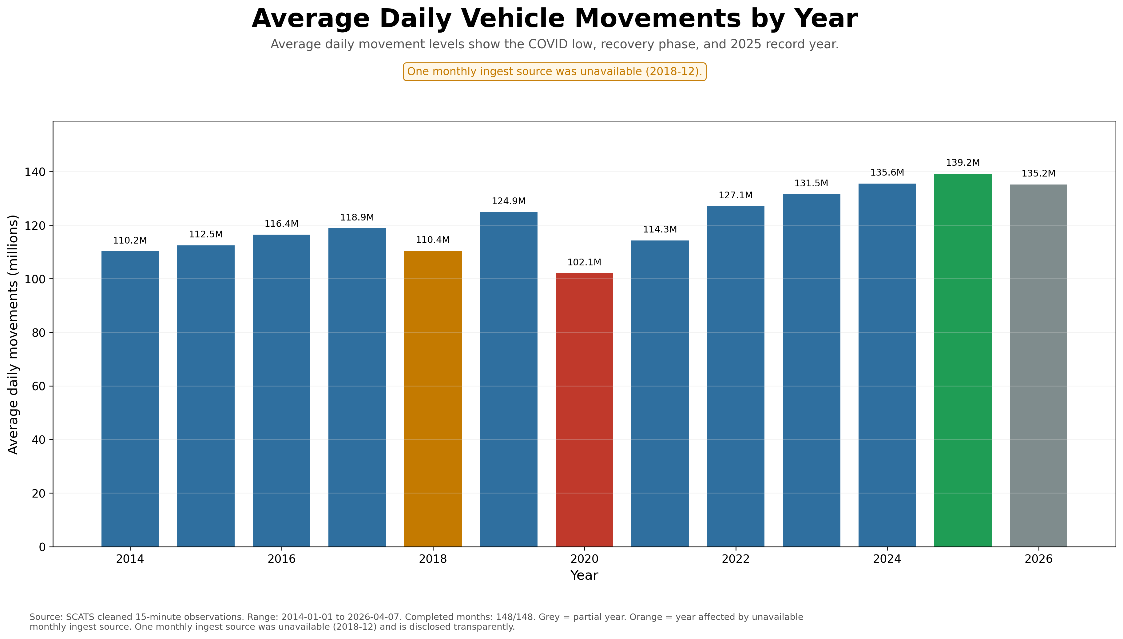
Record full year
2025
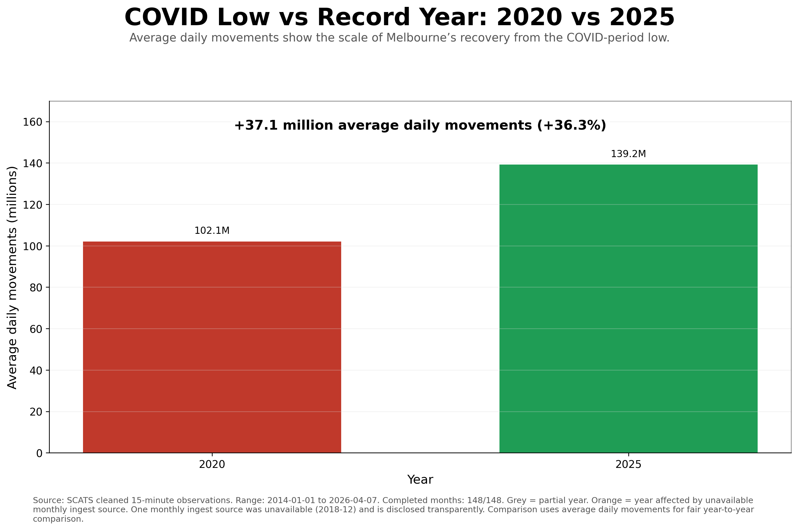
Approximately 50.5B movements and 139.2M average daily movements.
COVID-period low
2020
Approximately 37.0B movements and 102.1M average daily movements.
Recovery scale
+36.3%
2025 average daily movements compared with the 2020 low.
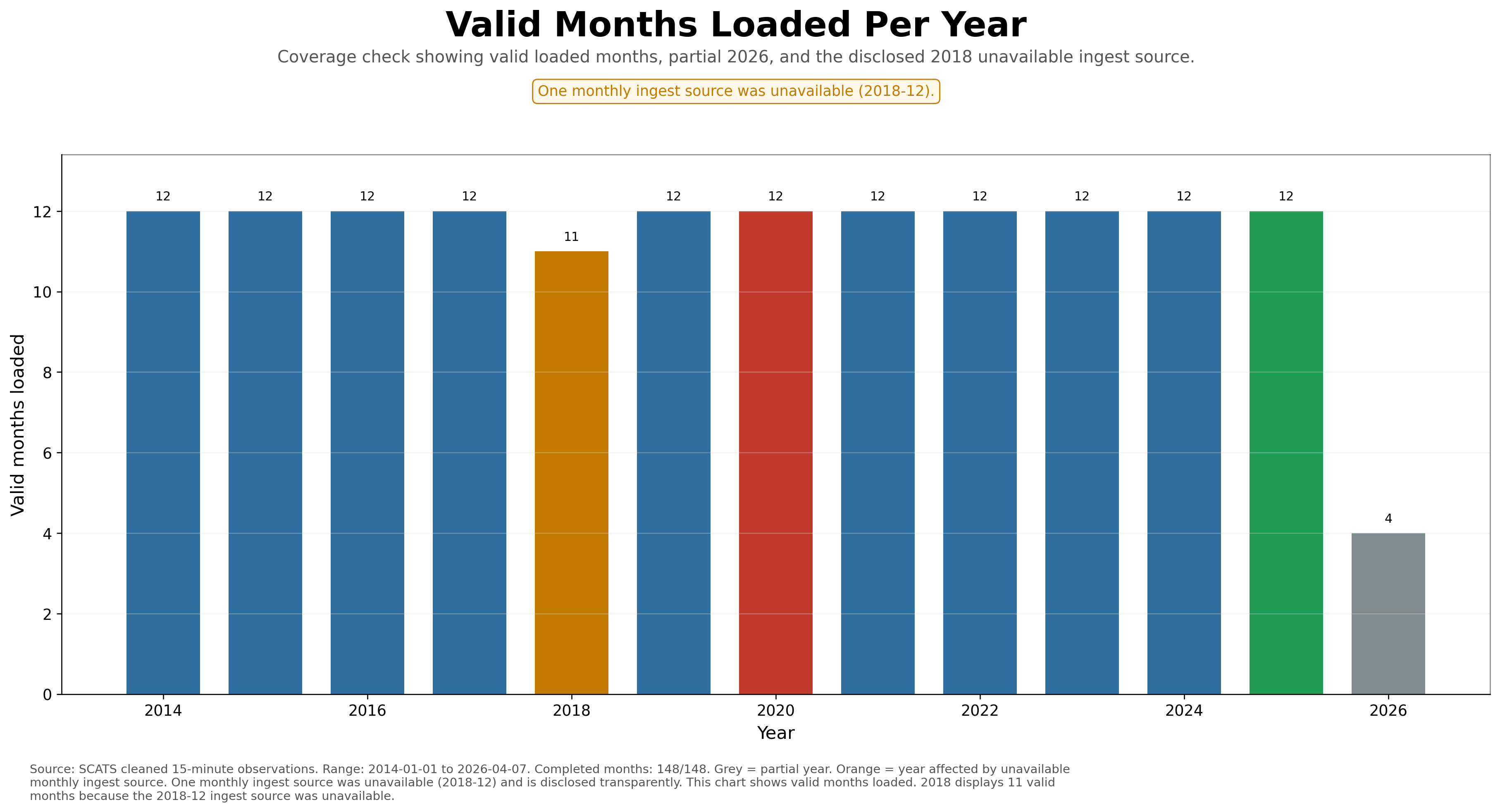
Coverage
148/148
All expected months in the reporting window were processed.
Partial year
2026
Shown separately as a partial year through 7 April 2026.
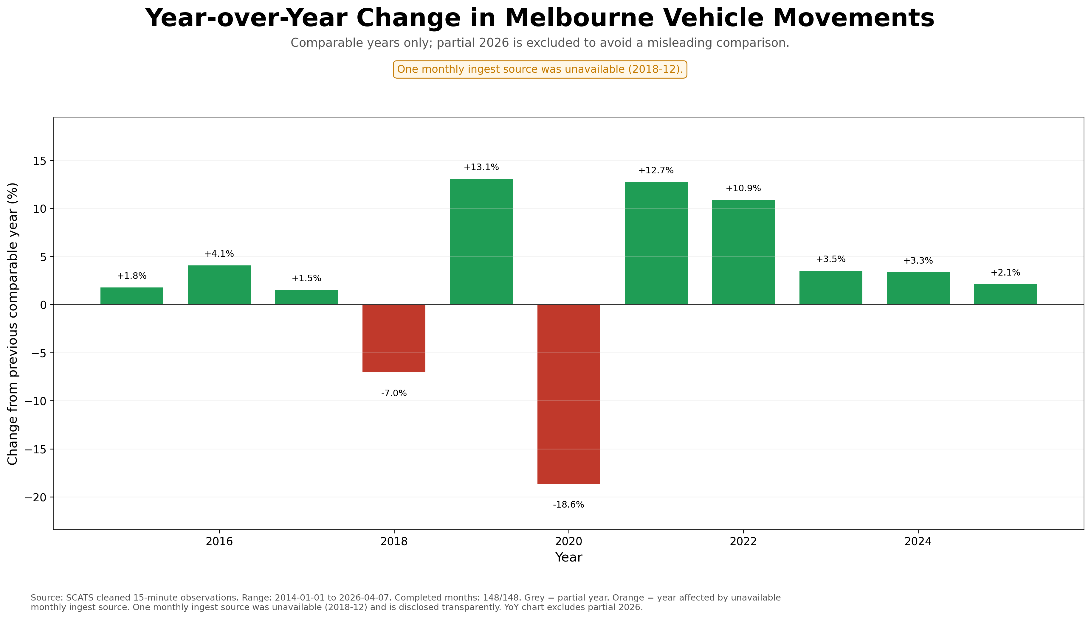
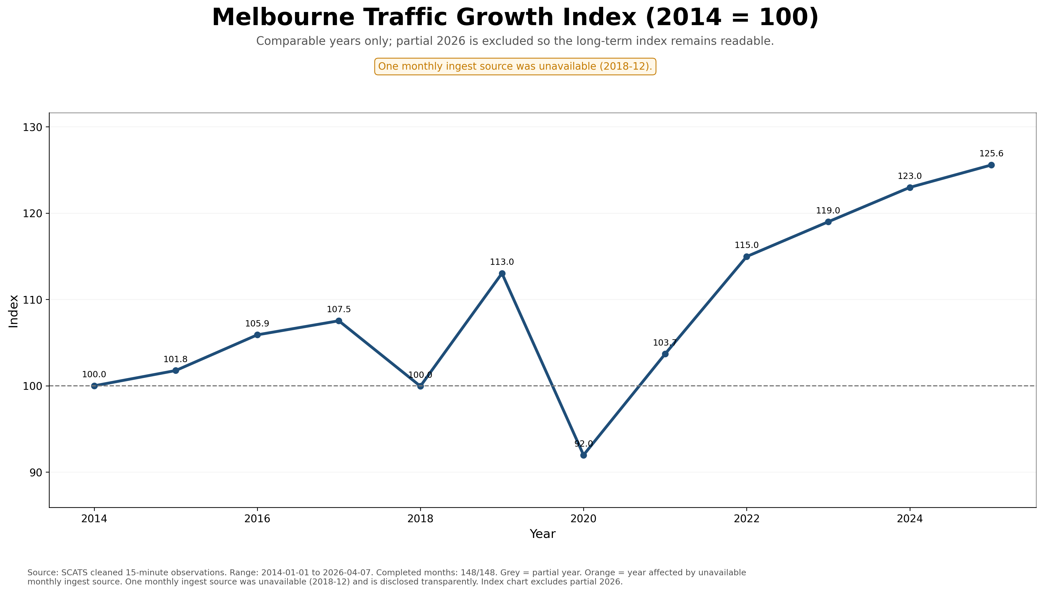
Data transparency note: One monthly ingest source was unavailable for 2018-12. The year is retained transparently in the charts and coloured orange where relevant. For fair trend comparisons, partial 2026 is excluded from year-over-year and indexed-growth charts.
1. Melbourne Total Vehicle Movements by Year
The flagship yearly chart. It shows the long-term traffic story: growth, COVID-period disruption, recovery, and 2025 emerging as the strongest full year.
This section gives the platform an executive-summary layer. The daily, monthly, site-level and 15-minute charts prove technical depth; the yearly totals explain the historical story in seconds. For journalists, government readers, OOH media, freight/logistics observers and the public, these yearly charts are likely to be among the most understandable and most frequently reused outputs on the page.
Confirmed result:
The completed monthly totals workflow confirms 539,020,710,239 cleaned vehicle movements across 148 / 148 months, covering the unified SCATS archive from 2014-01-01 to 2026-04-07. The run completed cleanly with 148 monthly CSV rows and the final JSON reports is_complete = true.
Total Cleaned Monthly Volume
539,020,710,239
Months Completed
148 / 148
Monthly CSV Rows
148
Date Range
2014-01-01 to 2026-04-07
Highest Volume Month
2025-10
Highest Monthly Volume
4,513,402,918
Lowest Month
2018-12
Lowest Monthly Volume
0 (missed/missing CSV file; not a true zero-traffic month)
Average Month
3,642,031,826
Median Month
3,704,917,910
Processing Time
4.54 hours
Workflow Status
Complete
This monthly result is now the backbone trend layer for the SCATS project. It gives the page a completed month-by-month time series that can feed the first major public charts: long-term monthly traffic, yearly totals, seasonal movement, pandemic-era disruption, post-pandemic recovery, and recent growth pressure.
Data-quality note:2018-12 is confirmed as a zero-volume month in the monthly output. That should be treated as a visible data gap or source-coverage issue, not as a real-world month with no traffic. The next-lowest non-zero month is 2026-04 with 840,492,772 cleaned vehicle movements.
Media interpretation: The strongest full month is 2025-10 with 4,513,402,918 cleaned vehicle movements. The completed yearly series shows the archive rising from approximately 40.23 billion cleaned movements in 2014 to 50.52 billion in 2025, making the monthly totals section one of the clearest ways to communicate long-term growth in Melbourne traffic demand.
Generated Monthly and Yearly Traffic Charts
Monthly Total Traffic
Long-term monthly cleaned traffic movement trend across the full SCATS archive.
Chart integration note: These images are loaded from the local charts/ folder created by generate_scats_charts_v3_9_colour.py. Keep this HTML file beside the charts directory when publishing or previewing the page.
Network monthly volume rebuilt from site-month totals
This V5.2 chart confirms the full network monthly trend from individual SCATS site-month rows, excluding the final partial month to avoid a misleading end-of-series drop.
Processing note: The final monthly totals JSON reports 148 / 148 months complete, 148 rows in the monthly CSV, and 16,326.969 total elapsed seconds. .
Confirmed Daily Totals Result
Confirmed result:
The completed daily totals workflow confirms 539,020,710,239 cleaned vehicle movements across 4,437 daily records, covering the unified SCATS archive from 2014-01-01 to 2026-04-07. The run completed cleanly with 148 / 148 months processed and is_complete = true.
Total Daily Volume
539,020,710,239
Daily Records
4,437
Months Completed
148 / 148
Date Range
2014-01-01 to 2026-04-07
Busiest Day
2025-12-12
Busiest Day Volume
166,208,622
Quietest Day
2025-05-27
Quietest Day Volume
7,556,689
Average Non-Zero Day
121,483,144
Median Non-Zero Day
124,567,849
Zero-Row Month
2018-12
Processing Time
4.39 hours
Daily totals are one of the most public-facing layers in the entire SCATS project. They allow the archive to move from technical database scale into clear city-history questions: Melbourne’s busiest traffic days, quietest disruption days, COVID-era collapse, holiday patterns, weekday/weekend behaviour, recovery curves, and the largest one-day shocks in the road network.
Important interpretation:2025-05-27 is currently the quietest non-zero day at 7,556,689 cleaned movements. Because it is dramatically lower than surrounding days, it should be treated as a high-priority investigation candidate before being presented as a real-world traffic collapse. The next day rebounds by approximately 140.3 million cleaned movements, which strongly suggests either a serious data coverage issue or an exceptional event that deserves separate checking.
Public-interest finding: The top 9 busiest daily records are all late-2024 to early-2026 dates, and 9 of the top 10 are Fridays. This gives the page a very simple public story: Melbourne’s highest measured daily SCATS volumes are heavily concentrated in recent years and around the end-of-week traffic cycle.
Generated Daily Traffic Charts
Daily Traffic Over Time
A full date-by-date line chart showing the complete daily movement spine from 2014 to 2026.
Chart integration note: These daily charts are loaded from the local charts/ folder created by generate_daily_totals_charts_v2_2_colour_annotated.py. Keep this HTML file beside the charts directory when publishing or previewing the page.
Top 10 Busiest Days by Total Cleaned Volume
Rank
Date
Day
Total Cleaned Volume
1
2025-12-12
Friday
166,208,622
2
2025-12-05
Friday
165,491,991
3
2025-11-28
Friday
165,193,216
4
2025-11-14
Friday
163,377,630
5
2025-11-21
Friday
162,975,898
6
2024-11-29
Friday
162,766,167
7
2024-12-13
Friday
162,314,859
8
2026-02-20
Friday
162,167,735
9
2026-02-13
Friday
162,114,953
10
2025-12-11
Thursday
161,713,728
Lowest 10 Non-Zero Days by Total Cleaned Volume
Rank
Date
Day
Total Cleaned Volume
1
2025-05-27
Tuesday
7,556,689
2
2020-08-09
Sunday
37,292,786
3
2020-08-16
Sunday
39,706,127
4
2020-04-10
Friday
40,210,106
5
2020-08-23
Sunday
41,090,426
6
2020-04-12
Sunday
41,621,250
7
2020-08-30
Sunday
43,273,397
8
2021-02-14
Sunday
45,418,017
9
2020-08-08
Saturday
45,858,809
10
2021-05-30
Sunday
46,547,102
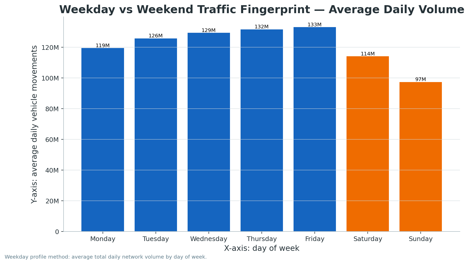
Average Daily Volume by Day of Week
Day
Daily Records
Average Cleaned Volume
Monday
633
119,397,506
Tuesday
635
125,719,289
Wednesday
634
129,360,318
Thursday
634
131,603,996
Friday
632
133,041,719
Saturday
634
114,018,602
Sunday
635
97,305,204
Processing note:
The final daily totals JSON reports 15796.017 total elapsed seconds,
equivalent to approximately 4.39 hours.
The source CSV path recorded by the workflow is
daily_totals.csv
.
Confirmed result:
The completed busiest-day process identifies 12 December 2025 as the busiest recorded traffic day in the unified SCATS archive, with 166,208,622 cleaned vehicle movements across the loaded network.
Busiest Day
2025-12-12
Busiest Day Volume
166,208,622
Daily Records
4,437
Quietest Non-Zero Day
2025-05-27
Day of Week
Friday
Total Volume
166,208,622
Date Range
2014-01-01 to 2026-04-07
Months Completed
148 / 148
Processing Time
31.5 hours
This is a simple, public-facing headline result: across more than twelve years of cleaned SCATS observations,
the highest single-day network total currently observed was Friday 12 December 2025.
The top-ranked days are strongly concentrated on Fridays, especially in late November and December, which points toward
end-of-year commuter, retail, logistics, and holiday-movement pressure.
Generated Busiest-Day and Weekday Charts
Top 10 Busiest Days
Ranked daily chart showing the highest recorded traffic days in the archive.
Interpretation note: The top daily results are dominated by recent years, particularly 2024–2026, which suggests the system is now capturing very high post-pandemic traffic demand. April 2026 remains a partial edge month because the archive ends on 2026-04-07.
Top 10 Busiest Days by Total Cleaned Volume
Rank
Date
Day
Total Volume
1
2025-12-12
Friday
166,208,622
2
2025-12-05
Friday
165,491,991
3
2025-11-28
Friday
165,193,216
4
2025-11-14
Friday
163,377,630
5
2025-11-21
Friday
162,975,898
6
2024-11-29
Friday
162,766,167
7
2024-12-13
Friday
162,314,859
8
2026-02-20
Friday
162,167,735
9
2026-02-13
Friday
162,114,953
10
2025-12-11
Thursday
161,713,728
Busiest Day by Year
Year
Busiest Date
Day
Total Volume
2014
2014-12-12
Friday
132,051,790
2015
2015-12-04
Friday
134,707,106
2016
2016-12-16
Friday
139,308,014
2017
2017-12-15
Friday
143,180,251
2018
2018-11-30
Friday
141,550,913
2019
2019-12-13
Friday
151,916,062
2020
2020-12-18
Friday
148,658,715
2021
2021-12-17
Friday
152,959,237
2022
2022-11-25
Friday
152,536,841
2023
2023-12-15
Friday
157,265,385
2024
2024-11-29
Friday
162,766,167
2025
2025-12-12
Friday
166,208,622
2026
2026-02-20
Friday
162,167,735
Processing note: The final busiest-day JSON reports the run as complete at 148 / 148 months. The V3 headline merge also confirms the busiest-day source as present and complete.
Confirmed Busiest Site Result
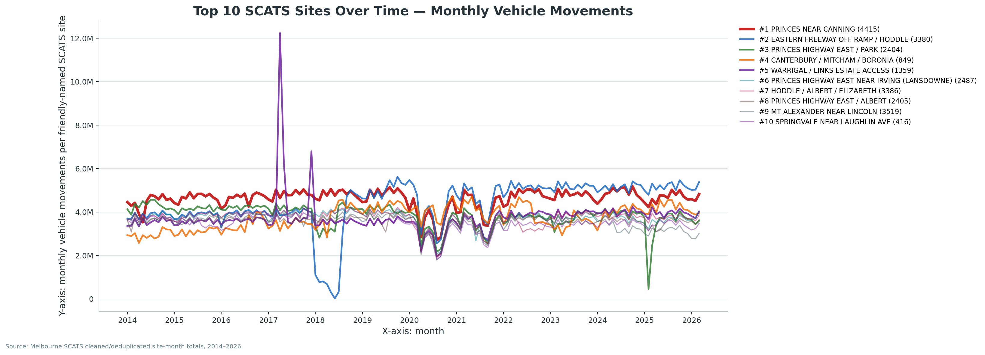
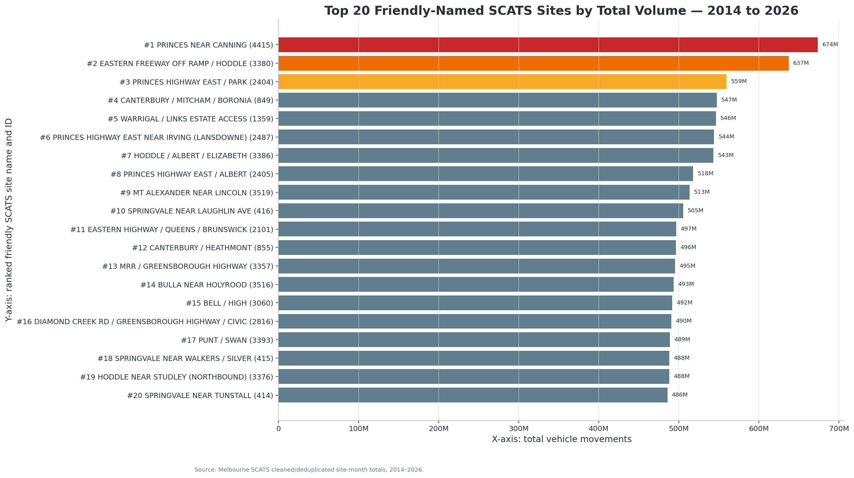
V5.2 site-month confirmation: The busiest-site result is now supported by a friendly-named Top 20 total-volume chart and a Top 10 over-time chart generated from site-month totals.
Confirmed result:
The completed busiest-site process identifies PRINCES NR CANNING (SCATS site 4415) as the busiest loaded SCATS location in the current archive, with 674,498,771 total cleaned vehicle movements across the loaded period from 2014-01-01 to 2026-04-07.
SCATS Site ID
4415
Site Name
PRINCES NR CANNING
Total Volume
674,498,771
Recorded Months
147
Peak Month
2024-10
Peak-Month Volume
5,171,583
Average Monthly Volume
4,588,427
Share of Total Cleaned Volume
0.125%
This is the first confirmed location-level headline result produced by the chunked site-ranking workflow.
It matters because it turns the project from a purely network-wide scale story into a place-specific intelligence story.
Readers can now point to a named SCATS site and say: this location carried more total cleaned traffic than any other currently loaded site in the archive.
Generated Busiest-Site Charts
Top 20 Busiest SCATS Sites
Ranked location chart showing the strongest loaded SCATS sites by total cleaned movements.
Interpretation note: The monthly CSV indicates that PRINCES NR CANNING was the top monthly site in 29 of the archive’s 148 processed month labels, while its strongest recorded month was 2024-10 with 5,171,583 movements. The low point of 927,843 in 2026-04 is a partial-month edge case because the archive ends on 2026-04-07.
Processing note: The final JSON summary reports the busiest-site run as complete at 148 / 148 months, with a total elapsed processing time of approximately 41.6 hours.
Confirmed Busiest Time Bin Result
Confirmed result:
The completed busiest-time-bin process identifies 17:15 as the busiest average daily network-wide 15-minute interval in the unified SCATS archive, with 10,133,657,484 total cleaned vehicle movements across 4,437 distinct dates. On an average day, that 15-minute interval alone recorded approximately 2,283,898 cleaned vehicle movements across the loaded network.
Busiest Time Bin
17:15
Total Volume in Bin
10,133,657,484
Distinct Dates
4,437
Average Daily Volume
2,283,898
Months Completed
148 / 148
Processing Time
46.8 hours
This result is especially useful for journalists because it gives the archive a simple, human-readable answer to the question: when is Melbourne's signalized road network busiest? The answer from this completed run is not a vague “PM peak”; it is a precise 15-minute bin: 5:15pm to 5:30pm.
Generated Time-of-Day Charts
Average Daily Traffic by Time of Day
Full 24-hour movement curve showing AM rise, PM dominance, and overnight low demand.
Method note: The ranking uses average daily volume per time bin, not raw total alone. That matters because it neutralises missed-day and partial-day distortion, especially around incomplete edge months such as April 2026.
Top 10 Time Bins by Average Daily Volume
Rank
Time Bin
Total Volume
Distinct Dates
Average Daily Volume
1
17:15
10,133,657,484
4,437
2,283,898
2
17:00
10,082,970,210
4,436
2,272,987
3
15:30
9,905,230,284
4,437
2,232,416
4
16:30
9,869,364,726
4,435
2,225,336
5
16:15
9,859,910,707
4,435
2,223,204
6
16:00
9,855,576,406
4,435
2,222,227
7
16:45
9,849,659,432
4,436
2,220,392
8
15:45
9,828,534,732
4,436
2,215,630
9
17:30
9,778,795,188
4,437
2,203,920
10
15:15
9,750,750,621
4,436
2,198,095
Monthly Winner Pattern
17:15: monthly winner in 108 months
17:00: monthly winner in 21 months
15:30: monthly winner in 17 months
15:15: monthly winner in 1 months
Interpretation
The top-ranked intervals cluster heavily around the afternoon peak.
17:15 dominates the monthly winner count, appearing as the top monthly bin in 108 months.
The top 10 list is almost entirely between 3:00pm and 5:45pm, confirming the strength and breadth of the PM peak.
Strongest Monthly Time-Bin Results
Month
Winning Time Bin
Monthly Volume
Distinct Dates
Average Daily Volume
2026-02
17:00
76,006,729
28
2,714,526
2025-10
17:15
83,961,729
31
2,708,443
2025-08
17:00
82,444,199
31
2,659,490
2024-05
17:00
82,236,304
31
2,652,784
2025-07
17:00
82,124,813
31
2,649,188
Processing note: The final JSON summary reports the busiest-time-bin run as complete at 148 / 148 months, generated at 2026-04-25 17:51:32 AEST, with a total elapsed processing time of approximately 46.8 hours.
Confirmed Quietest Time Bin Result
Confirmed result:
Using the completed monthly time-bin CSV, the quietest average daily network-wide 15-minute interval is 03:00, representing approximately 03:00–03:15. Across the loaded archive, this interval recorded 671,574,578 total cleaned vehicle movements across 4,437 distinct dates, averaging approximately 151,358 cleaned vehicle movements per day.
Quietest Time Bin
03:00
Approx. Time Window
03:00–03:15
Total Volume in Bin
671,574,578
Distinct Dates
4,437
Average Daily Volume
151,358
Source
Completed time-bin CSV
This result gives the page the natural counterpart to the confirmed busiest period. Together, the two results describe the daily movement envelope of Melbourne's signalized road network: the network is strongest around 17:15 and quietest around 03:00. That makes the story easier for a public audience to understand because it answers both ends of the same question: when does Melbourne move the most, and when does it move the least?
Generated Quietest-Time Chart
Top 24 Quietest Time Bins
Production-ranked overnight low-demand bins, using green intensity for quiet-network conditions.
Method note:
No new heavy DuckDB chunked run was required for this result. The completed
chunked_busiest_time_bin_monthly.csv
already contains every valid time bin by month, including monthly volume and distinct-date counts.
The quietest result is derived by aggregating those monthly rows and ranking by
average daily volume per time bin in ascending order, excluding blank placeholder rows.
Top 10 Quietest Time Bins by Average Daily Volume
Rank
Time Bin
Total Volume
Distinct Dates
Average Daily Volume
1
03:00
671,574,578
4,437
151,358
2
02:45
684,105,762
4,434
154,286
3
03:15
685,751,348
4,437
154,553
4
03:30
712,084,301
4,437
160,488
5
02:30
714,253,448
4,431
161,195
6
03:45
724,135,996
4,437
163,204
7
02:15
746,959,161
4,430
168,614
8
04:00
761,722,780
4,437
171,675
9
02:00
790,996,228
4,430
178,554
10
01:45
838,489,759
4,434
189,105
Monthly Quietest Pattern
03:00: monthly quietest bin in 127 months
02:45: monthly quietest bin in 15 months
02:30: monthly quietest bin in 4 months
03:45: monthly quietest bin in 1 months
Interpretation
The quietest intervals cluster tightly in the early morning sleep period.
03:00 is the lowest average daily interval across the full archive.
The top 10 quietest bins fall between roughly 2:00am and 4:15am, which is exactly the expected low-demand window for a metropolitan road network.
This result is a useful sanity check on the time-bin analysis because the quietest period lands where human behaviour predicts it should land.
Lowest Monthly Quietest Time-Bin Results
Month
Quietest Time Bin
Monthly Volume
Distinct Dates
Average Daily Volume
2020-08
02:30
2,180,259
30
72,675
2020-09
02:45
2,109,750
29
72,750
2021-09
02:45
2,404,575
30
80,152
2021-08
02:45
2,748,596
31
88,664
2020-04
02:45
2,574,004
29
88,759
Processing note: This section was derived from the completed busiest-time-bin monthly CSV, which contains 14,112 valid month/time-bin rows across the processed archive. The result should be treated as a confirmed derived output from the completed V3 time-bin workflow.
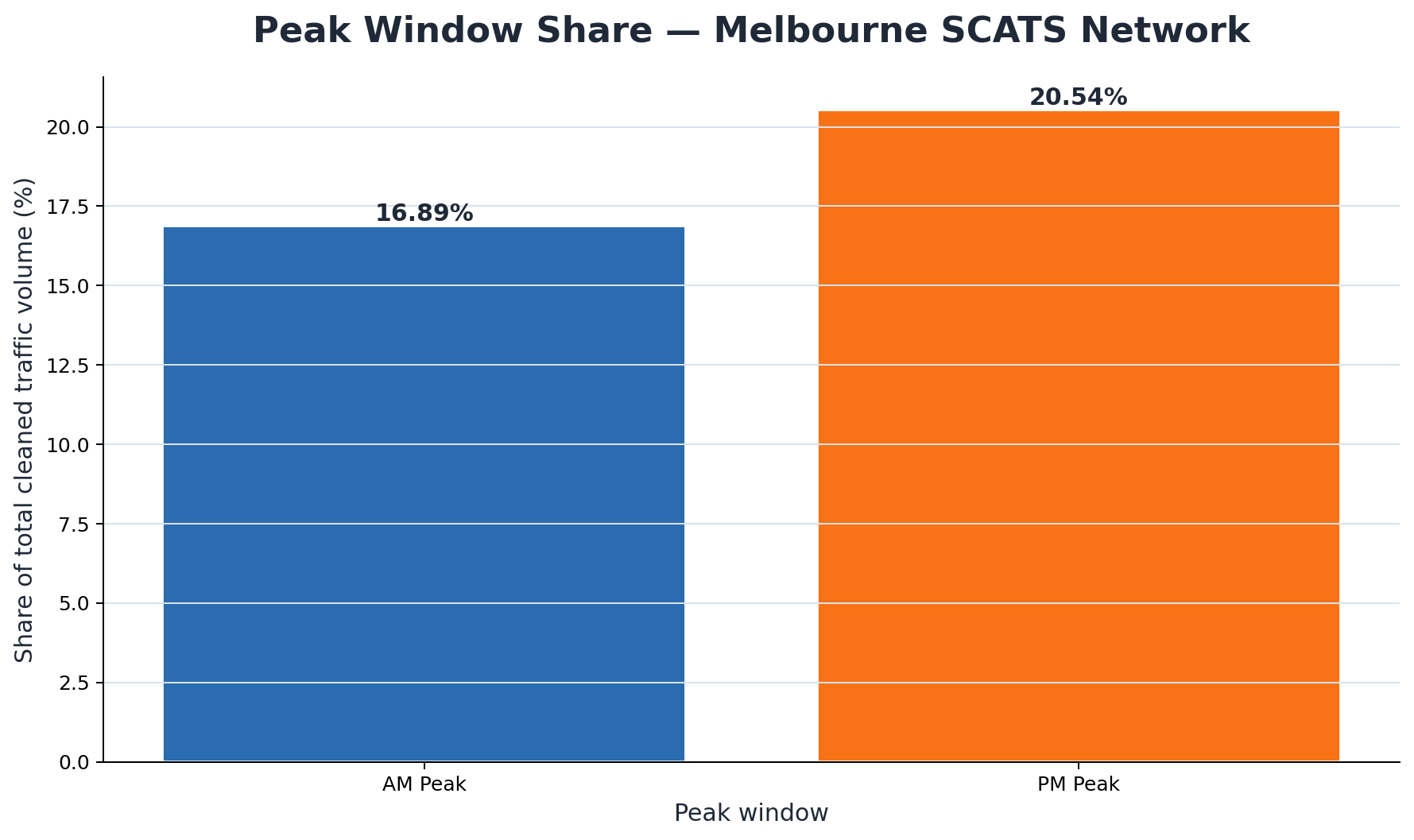
Confirmed Peak Share Results
Confirmed result:
The completed peak-share process confirms that 20.54% of all cleaned vehicle movements occur during the afternoon peak window (16:00–19:00), while 16.91% occur during the morning peak window (07:00–10:00). Across the full archive, the PM peak carries 110,696,055,470 cleaned movements and the AM peak carries 91,161,505,910 cleaned movements.
AM Peak Window
07:00–10:00
PM Peak Window
16:00–19:00
AM Peak Volume
91,161,505,910
PM Peak Volume
110,696,055,470
AM Peak Share
16.91%
PM Peak Share
20.54%
Combined Peak Share
37.45%
Total Volume Analysed
539,020,710,239
Months Completed
148 / 148
Processing Time
45.6 hours
Generated Peak-Share Charts
AM vs PM Peak Share Over Time
Monthly comparison of morning and afternoon peak shares across the archive.
This result shows that Melbourne's signalised road network is heavily concentrated into short daily demand windows. The afternoon peak is materially stronger than the morning peak, with approximately 19,534,549,560 more cleaned vehicle movements recorded in the PM peak than the AM peak across the archive.
Interpretation: Combined AM and PM peak windows account for 37.45% of all cleaned vehicle movements, even though they cover only six hours of the day. In plain English, nearly four in every ten recorded traffic movements occur during the two main peak windows.
Processing note: The final JSON summary reports the peak-share run as complete at 148 / 148 months, generated at 2026-04-27 18:54:10 AEST, with a total elapsed processing time of approximately 45.6 hours.
Simplified public weather layer:
This section focuses on Melbourne-wide SCATS network behaviour rather than individual site-level weather rankings. That keeps the public interpretation clear: the results show observed weather-associated traffic patterns across the network, not proof that weather alone caused changes at specific intersections.
The analysis joins trusted daily SCATS network totals from 2014-01-01 to 2026-04-07 with Bureau of Meteorology daily weather observations for rainfall, maximum temperature, minimum temperature and solar exposure. Days are grouped into practical weather classes such as rain, heavy rain, extreme rain, hot days, very hot days, extreme heat, cold mornings, sunny days and low-solar days.
Important interpretation note:
These figures are weather-associated network differences, not single-cause weather impacts. Rain, heat and sunshine can overlap with seasonality, weekday mix, school terms, public holidays, major events, roadworks, COVID-era disruption, local activity patterns and long-term traffic growth. The bottom line is: Melbourne-wide traffic volumes were historically higher or lower on days with these weather characteristics, but the weather classification should not be treated as the only cause.
What the headline numbers show
Melbourne’s weather story is more interesting than a simple “rain equals traffic chaos” headline.
At whole-network scale, ordinary rain is associated with only a modest traffic reduction, while
heavier rain, extreme rain, very hot days and low-solar days show clearer movement suppression.
In other words, Melbourne does not appear to shut down every time it rains — but the network does
respond when weather becomes more severe, gloomy or uncomfortable.
The warm-weather pattern is also revealing. Hot days above 30°C show a small positive network
difference, which may reflect stronger general activity, outdoor movement, retail activity,
beach and recreation travel, or seasonal effects. But once temperatures move into very-hot
territory, the pattern reverses: traffic volumes are lower than baseline. That suggests a practical
behavioural threshold where ordinary warm weather may support activity, while oppressive heat
begins to discourage or reshape travel.
Network-level weather response
The whole-network result suggests Melbourne traffic is resilient to ordinary weather but more
sensitive to uncomfortable or disruptive conditions. Rain days are only slightly below baseline,
but heavy rain and extreme rain show progressively larger reductions. Low-solar days also stand
out, which may capture the combined effect of grey, wet, cold or low-activity conditions rather
than sunshine alone.
This is useful because it separates everyday weather complaints from measurable network behaviour.
The data suggests that normal rain is not the same thing as a citywide disruption. The larger
movement changes appear when weather becomes severe enough to alter plans, reduce optional trips,
shift travel times or discourage discretionary movement.
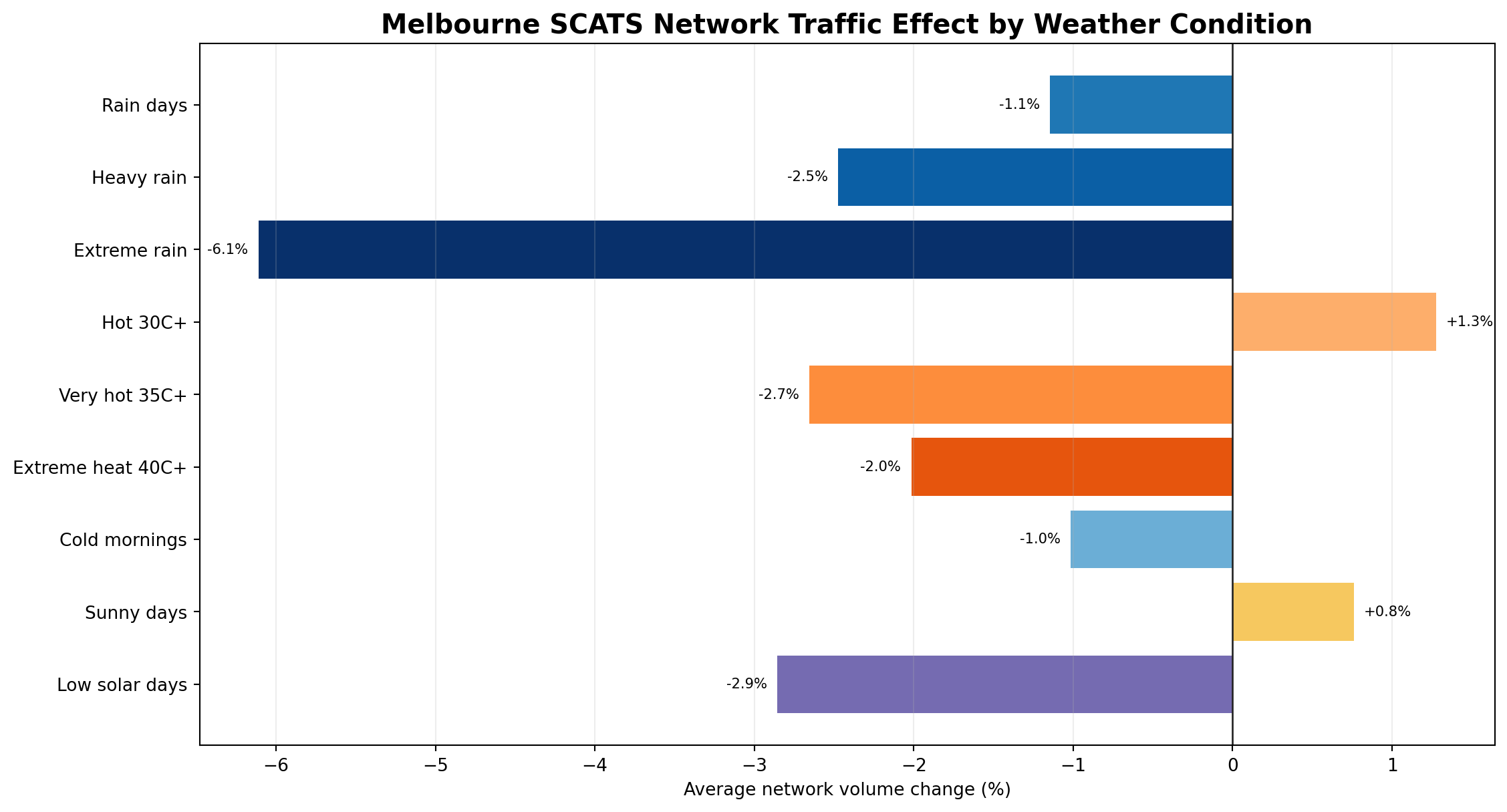
Melbourne-wide SCATS movement difference by weather condition. These are observed network differences versus baseline, not proof that weather alone caused the change.
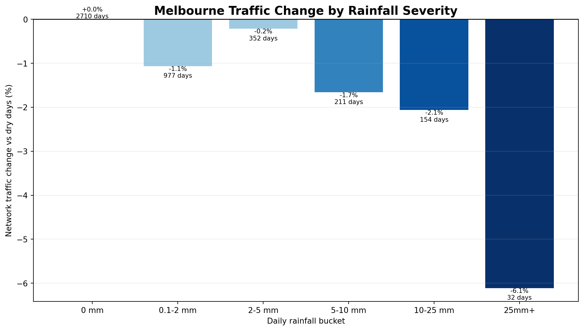
Rain severity matters
Melbourne talks about rain constantly, but the SCATS network does not treat all rain the same way.
Light or ordinary rain is associated with a relatively small movement difference. As rainfall
becomes heavier, the network-level reduction becomes more visible. That is the important public
finding: the traffic story is not simply whether it rained, but how severe the rain was.
A likely explanation is that light rain changes comfort more than necessity. People still commute,
go to school, make deliveries and move around the city. Heavier rain is different: visibility drops,
roads become less comfortable, minor incidents become more likely, some discretionary trips are
cancelled, and people may delay or consolidate travel. Extreme rain is where the citywide signal
becomes much clearer.
Rainfall bucket analysis showing how Melbourne-wide SCATS volumes differ as daily rainfall increases.
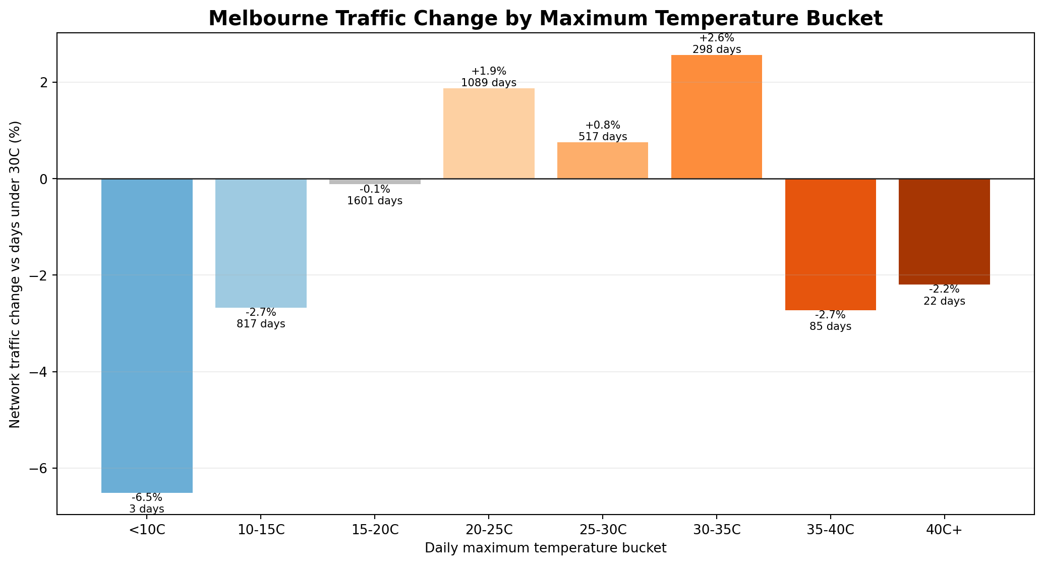
Temperature and heat behaviour
Heat behaves differently from rain. Warm and hot days can coincide with higher activity, especially
when people are still willing to travel for work, shopping, recreation, events or beach-related
movement. But very hot days appear to cross a behavioural threshold where movement falls below
baseline.
The extreme-heat result should be read carefully. Days above 40°C are much rarer than days above
35°C, so that bucket is more sensitive to weekday mix, school holidays, summer timing, public
holidays and unusual activity patterns. The safest interpretation is not that 40°C heat is “less
disruptive” than 35°C heat, but that very-hot weather shows the clearest negative network signal
in this version of the analysis, while extreme heat remains lower than baseline but is based on a
smaller and more variable sample.
Network traffic response by daily maximum temperature bucket, showing the difference between warm-day activity and very-hot-day suppression.
Why this matters
Melbourne has a cultural obsession with weather, but most weather-and-traffic discussion is based
on anecdotes: “the rain made traffic terrible,” “everyone stayed home because it was too hot,” or
“sunny days bring people out.” This analysis gives those claims a measured historical frame. It
does not prove weather alone caused the movement changes, but it shows that Melbourne-wide SCATS
volumes do vary in consistent, interpretable ways across different weather conditions.
The most useful finding is that weather response is graded, not binary. Ordinary rain is only
modestly different from baseline. Extreme rain is much more visible. Warm weather can coincide
with more activity. Very hot weather is associated with lower movement. Low-solar days also show
a meaningful reduction, suggesting that gloomy or low-light conditions may be part of a broader
low-activity weather pattern.
For journalists: the data turns Melbourne’s weather obsession into defensible numbers, showing which types of weather are actually associated with citywide traffic changes.
For road authorities: the result helps separate ordinary weather from conditions that deserve closer operational attention.
For freight and logistics operators: the network-level patterns can support planning around severe rain, very hot days and lower-reliability weather conditions.
For researchers: this creates a foundation for more controlled modelling using matched weekday, month, season, holiday and year baselines.
For the public: it shows that Melbourne traffic does not automatically collapse in all bad weather, but it does shift under more severe or uncomfortable conditions.
1. Weather data
Bureau of Meteorology daily observations were prepared for Melbourne, including rainfall, temperature and solar exposure.
2. Trusted SCATS daily totals
Network-level results use the existing trusted daily SCATS total file rather than re-summing site-level rows.
3. Weather classification
Days were classified into rain, heavy rain, extreme rain, hot, very hot, extreme heat, cold morning, sunny and low-solar categories.
4. Public interpretation
The public page now focuses on network-level weather-associated movement patterns, avoiding over-complex site-level claims that could be misread as direct causation.
Methodology note:
The network-level analysis uses trusted daily SCATS totals joined to daily Melbourne weather records. Results compare weather-classified days with the network baseline and should be interpreted as observed historical associations. Site-level V7 weather maps and charts were generated during analysis but are intentionally excluded from this public section because individual-site weather differences are more easily misunderstood without matched controls for weekday, month, season, events, holidays, roadworks, COVID-era disruption and local traffic changes.
Daily Melbourne SCATS network volumes were joined with Bureau of Meteorology weather-classified
days to identify broad, network-level traffic patterns associated with rain, heat, cold mornings,
sunshine and low-solar conditions. These figures show observed network differences, not proof
that weather alone caused the change.
🌧️
Rain days
−1.1%
Average network volume difference on rain-classified days versus the trusted SCATS daily baseline.
⛈️
Heavy rain
−2.5%
Heavier rain is associated with a larger observed drop in total Melbourne network movement.
🌊
Extreme rain
−6.1%
The strongest rain-classified days show the largest broad network traffic reduction.
☀️
Hot days 30°C+
+1.3%
Hot days show a small observed increase at the network level, likely mixed with season, activity, recreation and travel-pattern effects.
🔥
Very hot days 35°C+
−2.7%
Very hot conditions show the clearest negative heat-related network signal in this version of the analysis.
🥵
Extreme heat 40°C+
−2.0%
Extreme heat days show lower observed traffic, but the 40°C+ bucket is smaller and more sensitive to weekday mix, summer timing, holidays and unusual activity patterns.
❄️
Cold mornings
−1.0%
Cold-morning classified days are associated with a small reduction in network-wide daily movement.
🌤️
Sunny days
+0.8%
Sunny days show a small positive network difference, likely reflecting broader activity, seasonality and discretionary movement.
☁️
Low solar days
−2.9%
Low-solar days show one of the larger negative network-level differences outside extreme rain, possibly capturing gloomy, wet or low-activity conditions.
Interpretation note:
These are weather-associated traffic patterns, not weather-only causal claims.
Weather-classified days can also overlap with seasonality, weekday mix, school terms,
public holidays, major events, roadworks, COVID-era disruption, local activity and long-term traffic growth.
Spatial view:
This interactive Google Map plots the top 20 busiest SCATS sites by total cleaned vehicle movements. Friendly public-facing names are shown first, while official SCATS labels and site IDs remain visible for auditability.
Mapped Sites
20
Busiest SCATS Site
4415
Top SCATS Site Volume
674.5M
Lowest SCATS Top-20 Volume
486.3M
Friendly names
Main road / cross road / local landmark, with direction added where it matters.
Official traceability
Each popup and table row keeps the SCATS site ID and official SCATS label.
Corridor grouping
Sites are grouped into readable arterial corridor categories for non-technical readers.
Traffic Intensity Legend
Red — Extreme traffic load
Orange — Very high traffic load
Yellow — High traffic load
Green — Lower within top 20
Circle size is scaled by total cleaned vehicle movements. Labels show rank order.
Key observation: The map shows strong clustering around the inner Melbourne, Hoddle, Eastern, Princes, Springvale, and north-eastern arterial corridors. This turns the ranked table into visible geographic traffic intelligence.
Interactive Map Site Directory
Rank
Friendly Location Name
SCATS ID
Corridor Group
Total Movements
Heat
Google Map
1
Princes Highway near Canning Street Official SCATS label: PRINCES NR CANNING
Top 20 Busiest SCATS Sites — Human-Readable Directory
Naming convention:
Each site is shown as a plain-English road location first, followed by the official SCATS site ID and original SCATS label. Slashes indicate intersecting roads or joined road approaches. Where the original label uses NR, the readable name converts it to near. Where the site has latitude/longitude coordinates, the map link opens directly at the mapped point; where coordinates are missing, the map link opens a Google Maps search using the SCATS ID and site name.
Why this matters: SCATS labels are useful to engineers but not ideal for public readers. This directory turns the top-ranked traffic sites into recognizable Melbourne locations while preserving the exact SCATS ID for auditability.
Rank
Reader-friendly location name
SCATS ID
Official SCATS label
Total movements
Map target
Google Map
1
Princes Street near Canning Street Inner-north arterial hotspot
Manual name overrides used: SCATS site 2816 is shown as Diamond Creek Road / Greensborough Highway / Civic Drive, and SCATS site 3376 is shown as Hoddle Street near Studley Park Road — northbound. These two labels fill gaps left by the first coordinate lookup table.
Interactive Map — Full Melbourne SCATS Site Network
Full network explorer:
This section expands beyond the Top 20 sites and plots every mapped SCATS site with valid coordinates. Readers can search by SCATS ID, road name, municipality, or traffic band, then scroll through the full site directory without the page becoming dominated by thousands of rows.
Mapped Sites
4,427
Top SCATS Site
4415
Top SCATS Site Volume
674.5M
Traffic Bands
4
Reader use case: The Top 20 map is ideal for headline hotspots. This full-network map is better for suburb-by-suburb exploration, local reporting, OOH media planning, and letting readers find intersections they personally know.
Scrollable Full SCATS Site Directory
The full directory is intentionally contained in a scrollable box so readers can browse thousands of mapped sites without making the page unusably long.
Loading all sites…
Rank
SCATS Site
ID
Municipality
Total
Map
Traffic Intensity Legend
Red — Top 5% busiest sites
Orange — Top 20% busiest sites
Yellow — Middle-volume sites
Green — Lower-volume mapped sites
Circle size is scaled lightly by volume. Colours are based on percentile rank among sites in the cleaned archive.
Full Map Controls
Showing all mapped sites.
Interactive Map — Melbourne SCATS Site Changes After the West Gate Tunnel Opening Period
New citywide post-tunnel visual intelligence layer:
This embedded Google Map compares SCATS-detected vehicle movements at mapped signal sites for
Jan–Mar 2025 versus Jan–Mar 2026. Red/orange markers indicate sites where detected traffic increased, blue markers indicate sites where detected traffic decreased, and grey markers indicate sites that were roughly flat.
Mapped Sites
4,343
Comparison Period
Jan–Mar
Net Change
+257.6M
Overall Change
+2.15%
Reader use case: This map is designed for journalists, councils, transport analysts and residents who want to visually inspect where monitored traffic volumes rose or fell after the West Gate Tunnel opening period. It is not a truck-only map; SCATS counts total detected movements at signalised sites.
How to read the map:
Red/orange = detected traffic increased between Jan–Mar 2025 and Jan–Mar 2026.
Blue = detected traffic decreased between Jan–Mar 2025 and Jan–Mar 2026.
Grey = roughly flat, within approximately ±3%.
Larger circles = larger traffic sites, scaled using the larger of the two Jan–Mar totals.
Click a site marker to see the SCATS site name, site ID, before/after totals, absolute change, percentage change, historical total and Google Maps link.
Method note: The map is a preliminary site-level SCATS comparison. It compares total SCATS-detected vehicle movements, not truck-classified movements. Individual site changes may reflect traffic redistribution, roadworks, detector configuration changes, signal changes, local network changes or genuine demand shifts. The map is best read as a powerful investigative layer showing where further analysis is needed.
Network Coverage Map
The coverage layer now spans full SCATS network coverage, ranked busiest SCATS sites, Top 20 mapping, temporal behaviour, site-month intelligence, corridor dominance, parcel/OOH opportunity mapping, Kepler movement visualisations, COVID/recovery intelligence and reproducibility evidence.
West Gate Bridge and freeway corridor references should be read together with the TIRTL analysis page: West Gate traffic analysis.
Strategic interpretation: this is now an independent Melbourne movement intelligence platform. SCATS explains the signalised network at scale, the parcel layer connects exposure to commercial land opportunity, and future TIRTL integration will deepen freeway, speed, class and heavy-vehicle intelligence.
Kepler.gl Spatial Traffic Intelligence Maps
New spatial intelligence layer:
The SCATS analysis now includes exported Kepler.gl WebGL maps built from the cleaned site-volume and coordinate dataset. These maps move the page beyond charts and tables by showing Melbourne traffic as a geographic intensity field: the full network, the arterial backbone, and the highest-ranked critical traffic nodes.
The exported map layers below form a progressive traffic-intelligence hierarchy. Readers can begin with the full SCATS network, zoom into the CBD, narrow to the top 5% busiest arterial backbone, then isolate the top 1% most critical traffic nodes. This turns the SCATS archive into a spatial tool for journalists, planners, councils, researchers, and commercial analysts.
Full network viewShows the complete mapped SCATS signal network and validates the geographic coverage of the dataset.
Top 5% arterial backboneRemoves lower-intensity noise and reveals Melbourne's major movement corridors.
Top 1% critical nodesIdentifies the highest-ranked traffic pressure points likely to matter most during incidents and disruptions.
Future animation baseThese maps establish the spatial foundation for future month-by-month and time-of-day Kepler.gl animations.
Static export set
Full Metro Traffic Intensity
The complete Melbourne SCATS network rendered as a weighted traffic intensity field. This is the baseline geographic view of the system.
This highest-pressure node view isolates the most critical 1% of mapped SCATS sites, showing the locations most likely to matter during congestion, incidents, and network disruption.
New critical-network exports: The Top 5% arterial backbone and Top 1% critical nodes maps show the difference between Melbourne's broad traffic structure and its highest-pressure failure points. Place both PNG files in the local charts/ directory beside the other generated charts.
Interactive Kepler.gl exports
All SCATS Sites Master Map
Interactive WebGL map showing all mapped SCATS sites with hover tooltips, volume scaling, and geographic coverage across Melbourne and surrounding regions.
This embedded preview loads the exported Kepler.gl map. If it does not display when opened locally, open the linked HTML file directly or host all exported files in the same web directory as this page.
Publishing note: The exported Kepler.gl HTML files should be uploaded beside this page, along with the three PNG map exports. The Kepler.gl exports may include a Mapbox access token in plain text; restrict any production token by domain before publishing publicly.
Cinematic SCATS Traffic Animations
These click-to-play videos turn the completed Melbourne SCATS analytics into short cinematic movement films.
They combine generated traffic animations with soundtrack layers so the data can be understood visually and emotionally, including the weekly heartbeat of Melbourne, local 7-day pulse rendering, Kepler.gl 24-hour time-bin playback, daily rhythm, seasonal behaviour, full-network coverage, Top 100 sites and COVID collapse/recovery history.
Playback note: Videos are embedded with standard browser controls and do not autoplay. Click play on any video to start it.
Melbourne Weekly Traffic Heartbeat
A cinematic day-of-week animation showing Melbourne’s weekly SCATS traffic rhythm: Monday’s weaker restart, the workweek build-up, Friday’s maximum movement intensity, and the sharp weekend fall into Sunday rest-state traffic.
A cinematic full-network reveal of Melbourne’s mapped SCATS signal sites, showing the geographic scale of the system before the page drills into daily, seasonal, time-bin and Top 100 intelligence.
A locally rendered Python/ffmpeg animation of the 7-day Melbourne SCATS pulse, showing one frame per 15-minute bin across the full week without relying on Kepler.gl playback.
An OBS-recorded Kepler.gl animation of Melbourne’s SCATS network across a full 24-hour cycle, stepping through 15-minute time bins so viewers can watch the city wake, surge, peak, release and quieten again on the map.
A cinematic seasonal animation showing Melbourne’s month-of-year traffic rhythm, including the January trough and high-intensity February/November behaviour.
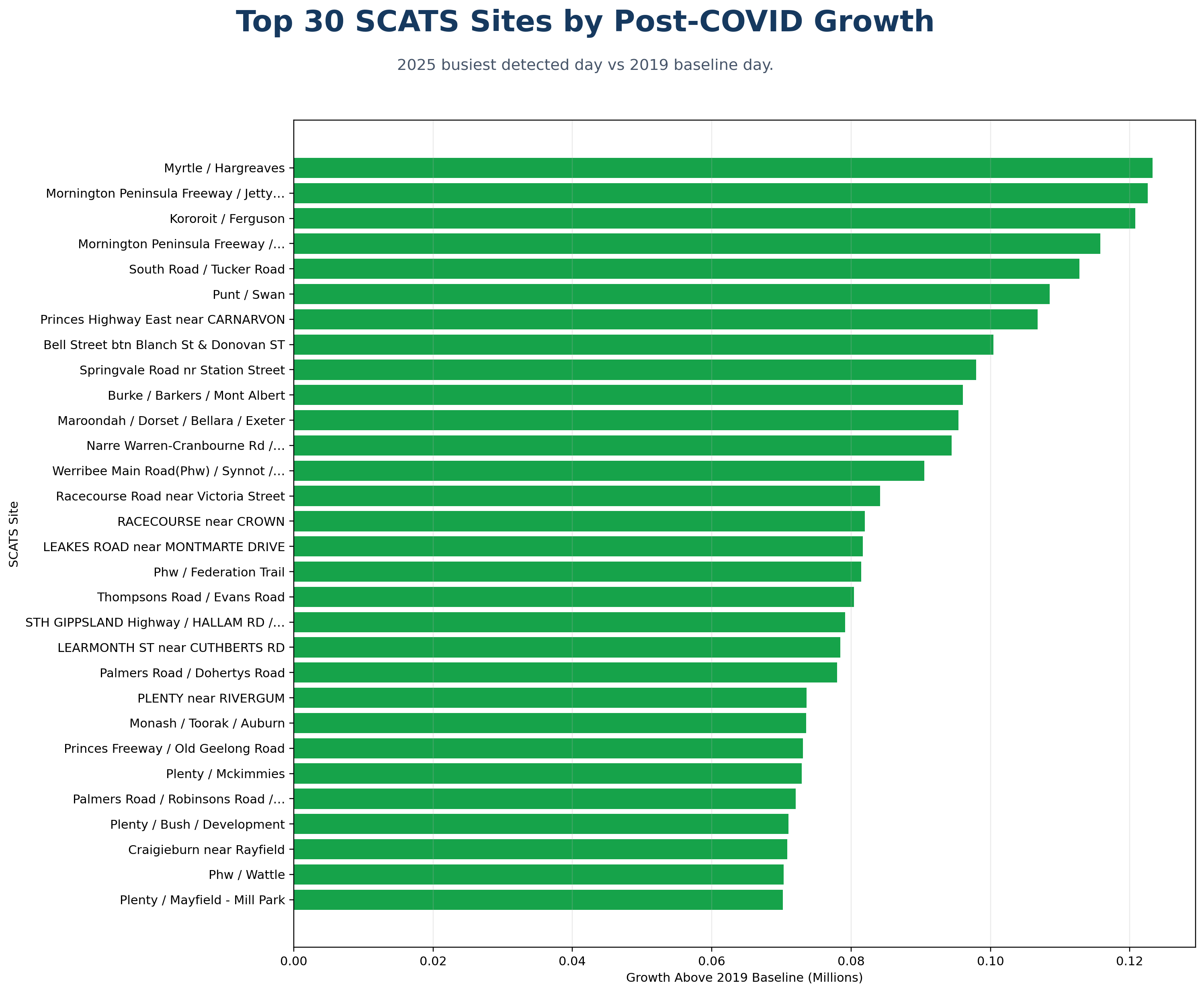
A cinematic citywide map animation showing Melbourne traffic moving from the 2019 baseline through lockdown shock, disruption, recovery, recent normal and the 2025 busiest detected day.
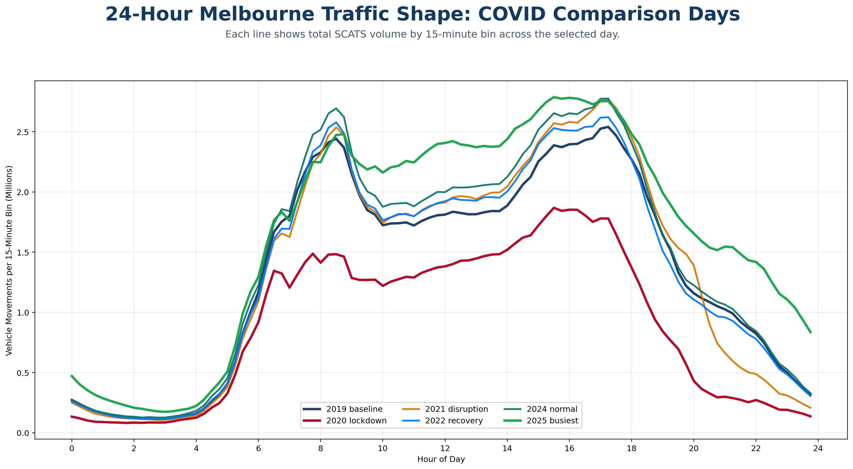
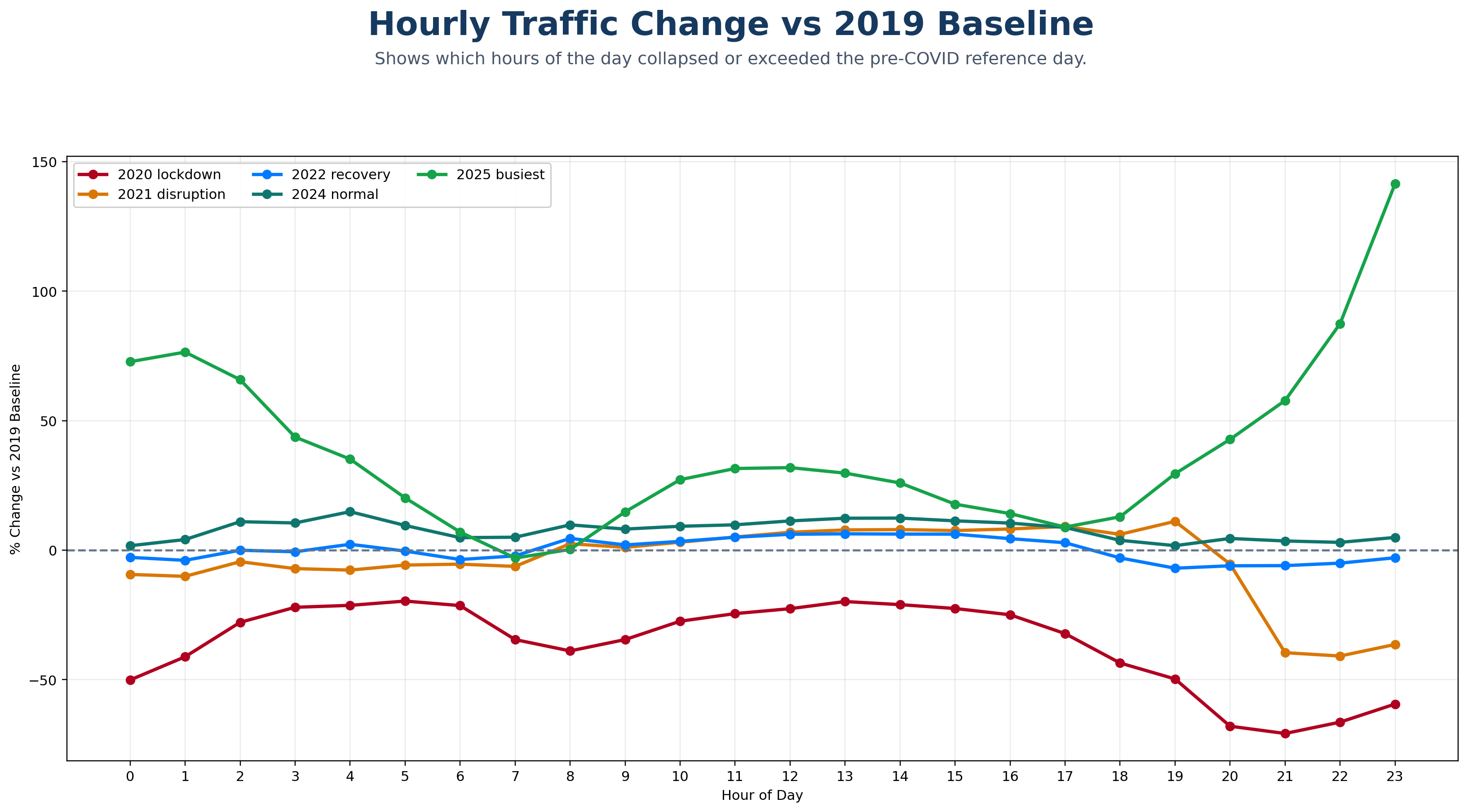
An animated 24-hour curve comparison showing how Melbourne’s daily traffic rhythm collapsed during lockdown and then rebuilt across later recovery periods.
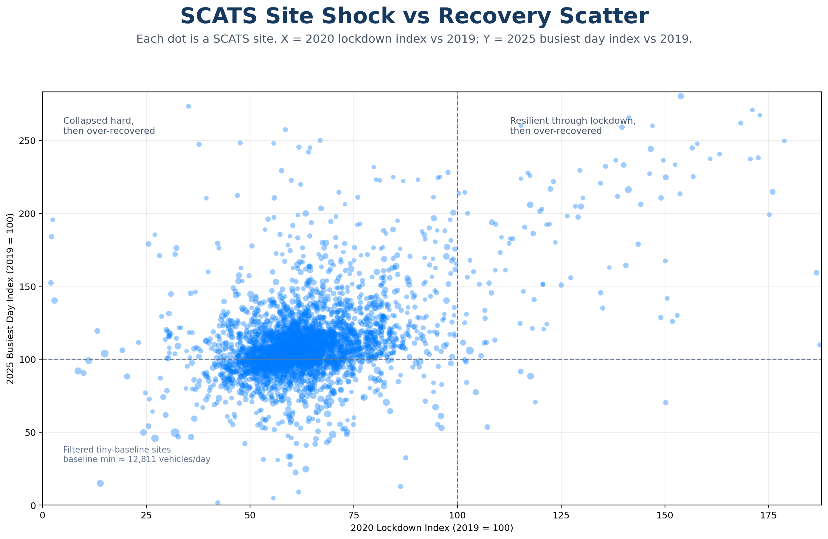
A site-level resilience animation revealing which SCATS nodes collapsed hardest during lockdown and which later over-recovered beyond the 2019 baseline.
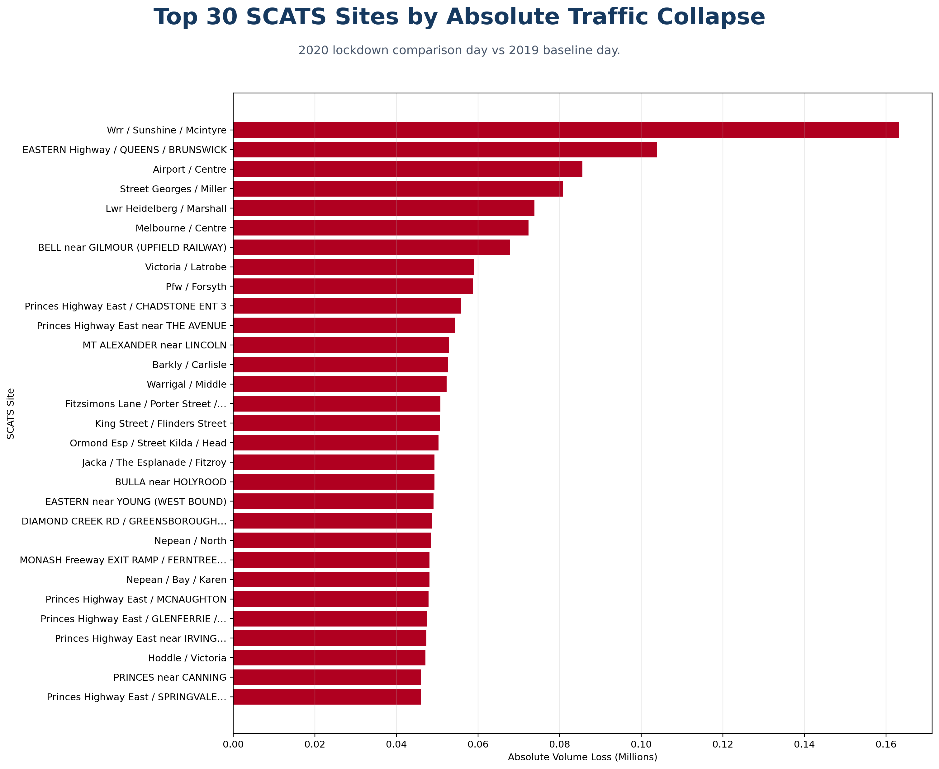
An animated leaderboard of the SCATS sites with the largest absolute traffic-volume losses on the 2020 lockdown comparison day versus the 2019 baseline.
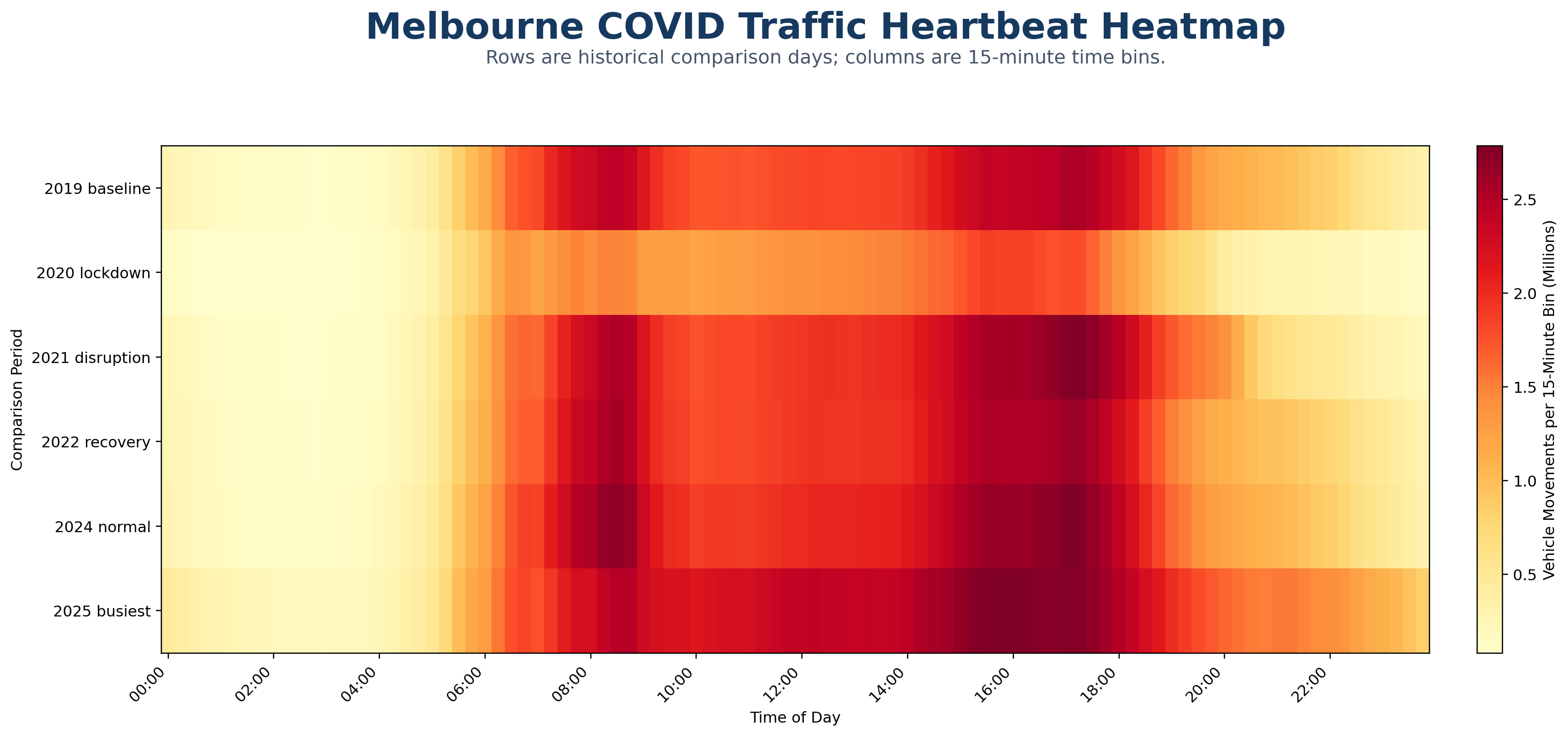
A row-by-row reveal of the COVID comparison heatmap, showing how the 15-minute daily traffic signature changed from baseline to lockdown, recovery and overperformance.
Why this matters: The animations make the SCATS archive easier for journalists, policy readers, advertisers and the public to understand.
Instead of presenting only numbers, the page now shows Melbourne as a living movement system across weekly heartbeat behaviour, full-network coverage, daily volume, seasonal behaviour, time-of-day rhythm, COVID collapse/recovery history and commercial-location dimensions.
Find Your Melbourne Suburb Traffic Profile
Search the suburb-level Melbourne SCATS Intelligence reports. Each profile links to a full web report
and a downloadable PDF generated from the same mapped SCATS suburb movement layer.
Start typing to generate report links. Search results below can also be clicked to populate the report buttons.
The Melbourne Suburb Traffic Intensity Map adds a suburb-level visual layer to the SCATS project. Instead of only reading suburb tables and Top 100 rankings, users can now explore Melbourne geographically and see how traffic pressure varies across suburbs.
Red, yellow and green suburb traffic pressureInteractive suburb polygons joined to cleaned SCATS traffic-pressure scores
Suburbs are colour-coded by observed traffic pressure so people can quickly see high, medium and lower traffic-intensity areas.
How it was built
Cleaned SCATS suburb traffic-pressure scores were joined to suburb-level GeoJSON boundary polygons and rendered as an interactive map layer.
Why it matters
The Top 100 list shows rankings; the map shows geography. It helps people visually understand where traffic pressure clusters across Melbourne.
Interpretation note: This is a signalised-traffic pressure map, not a count of every vehicle on every street. It is strongest where SCATS signal coverage is good. A suburb with fewer monitored signalised intersections may appear quieter than local experience suggests.
The Melbourne Commute + Traffic Pressure Map combines modelled CBD commute estimates with the existing SCATS suburb traffic-pressure layer. It is designed for people asking practical questions such as: how bad is my commute, how much worse is peak hour, and how does my suburb compare with nearby suburbs?
Suburb-centroid estimates include AM peak commute to the CBD, PM return from the CBD, off-peak travel time and peak-delay penalty.
Traffic pressure
The commute layer is combined with SCATS suburb traffic-pressure scores, so the map does not only show travel time — it also reflects local traffic load.
Comparison metrics
The map supports practical comparison through traffic pain index and low-traffic / high-access scoring.
Interpretation note: Commute times are modelled suburb-centroid drive-time estimates. They are useful for comparing suburbs, but they are not exact driveway-to-work predictions. Individual addresses, incidents, roadworks and daily conditions will vary.
Melbourne Commute + Traffic Pressure Graphs — Version 2
These Version 2 graphs summarise the suburb commute intelligence output using a metro-style filter. They show the fastest and slowest CBD commutes, PM return pressure, peak-delay penalties, traffic pain, low-traffic / high-access scoring, commute-time distributions and scatter plots connecting commute time, traffic pressure and route distance.
Version 2 filter note: Public charts are metro-filtered by default to avoid regional Victorian localities appearing in Melbourne suburb rankings. The commute times are modelled suburb-centroid estimates and should be used for suburb comparison, not exact address-level trip prediction.
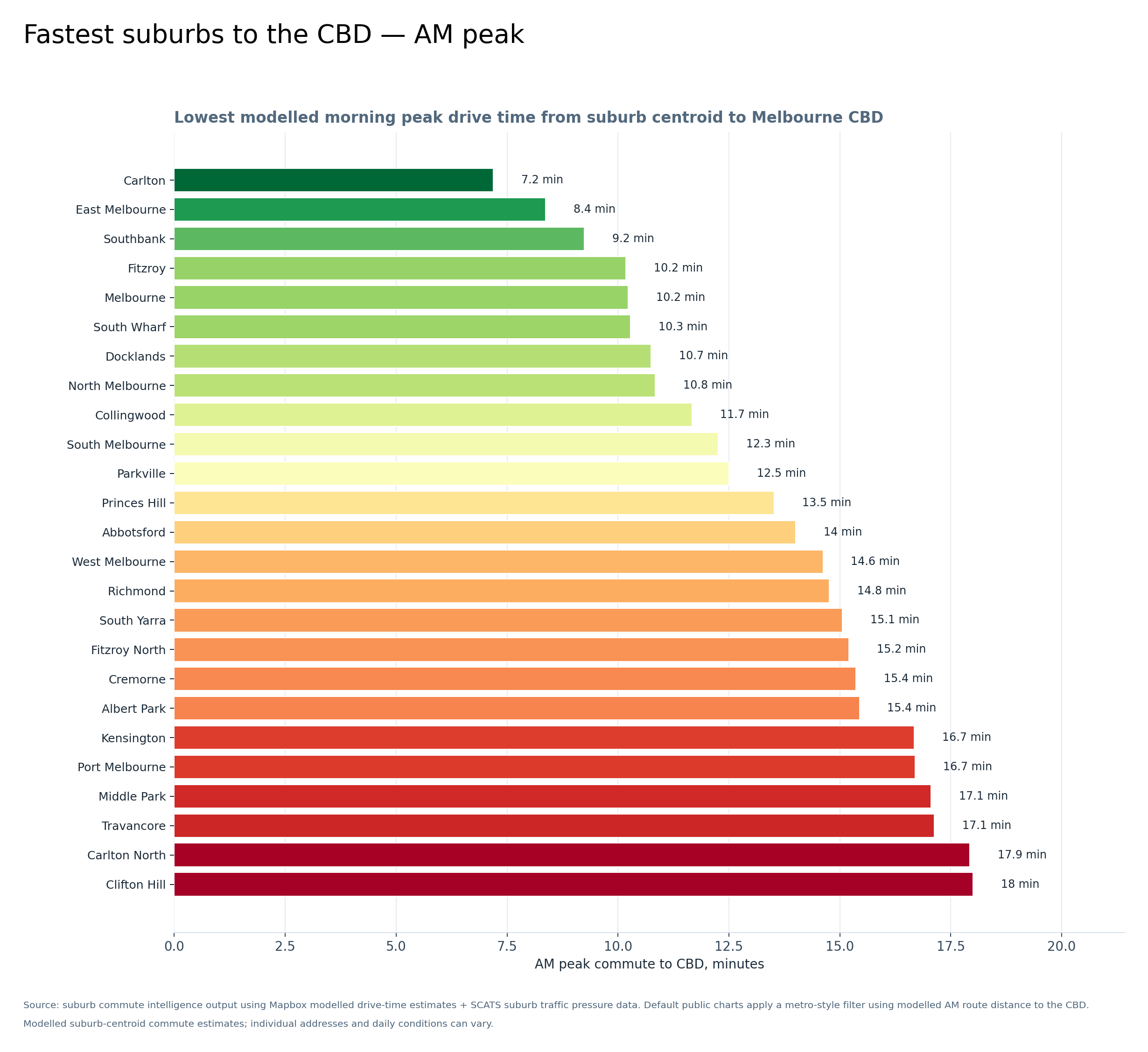
Graph 1 — Fastest suburbs to the CBD, AM peak
This graph shows the fastest modelled morning peak CBD commutes from suburb centroids. The inner suburbs dominate: Carlton, East Melbourne, Southbank, Fitzroy, Melbourne, South Wharf, Docklands and North Melbourne all sit close to the CBD and perform strongly.
Modelled suburb-centroid drive-time estimates; individual addresses and daily conditions will vary.
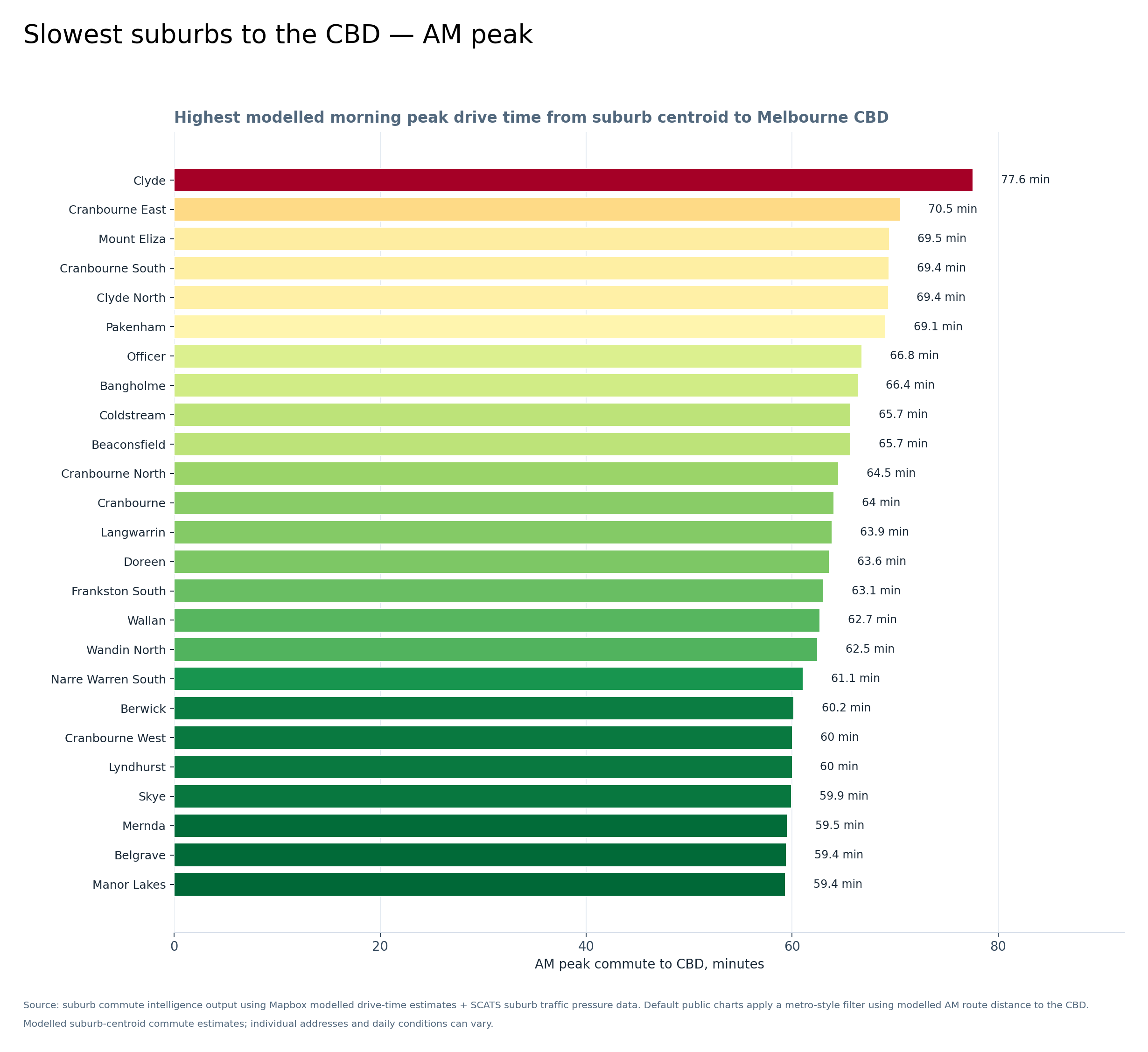
Graph 2 — Slowest suburbs to the CBD, AM peak
This is where the commute-pressure story becomes very clear. Clyde, Cranbourne East, Clyde North, Pakenham, Officer, Beaconsfield, Berwick and surrounding growth-corridor suburbs appear near the top.
The south-east growth corridor stands out strongly in the modelled AM peak commute data.
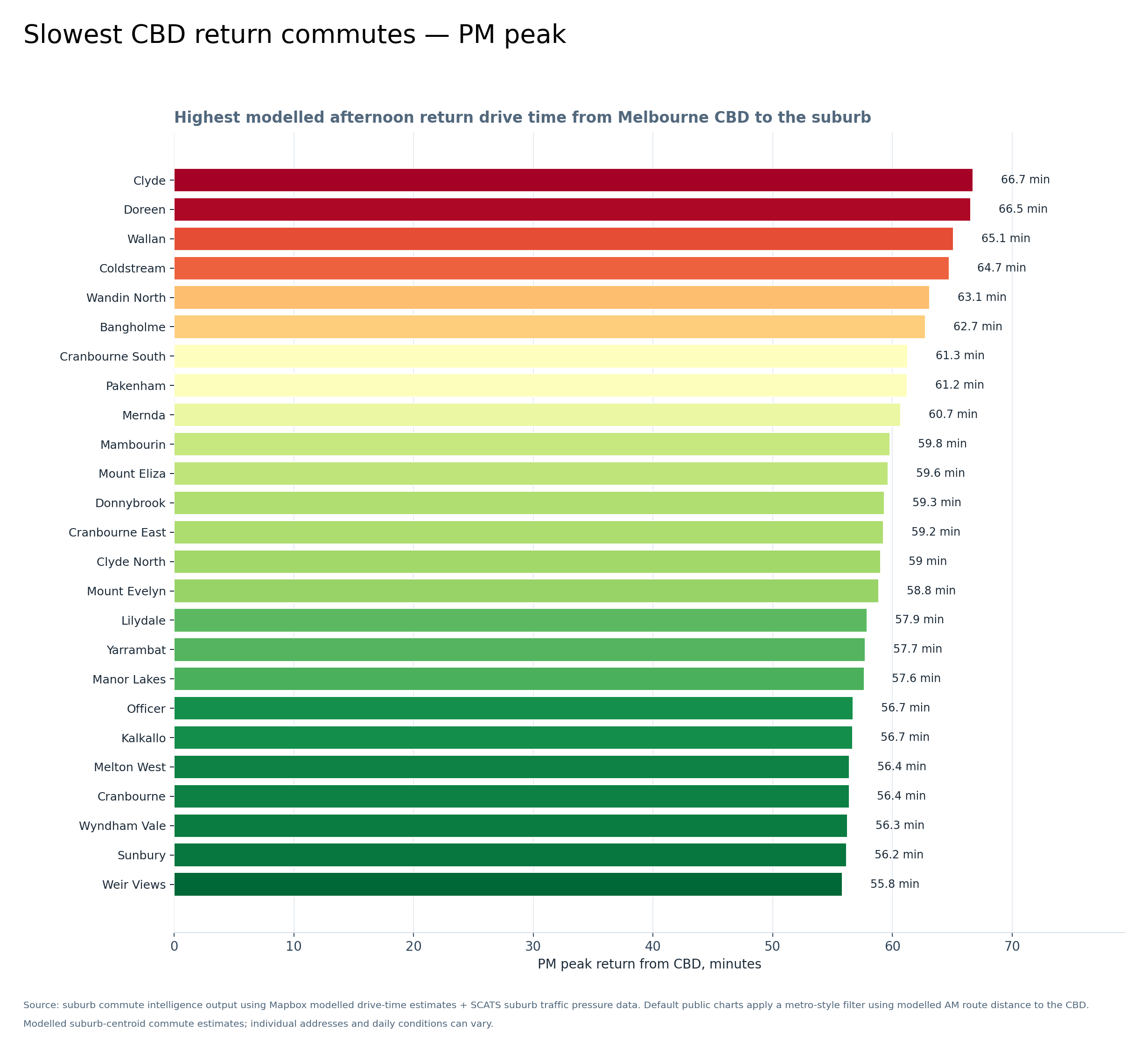
Graph 3 — Slowest CBD return commutes, PM peak
This graph looks at the afternoon return trip from the CBD back to each suburb. The outer growth areas again show up strongly, especially Clyde, Doreen, Wallan, Coldstream, Pakenham, Mernda, Donnybrook and the Cranbourne/Clyde corridor.
Commute pressure is not just about getting into the city — the trip home matters too.
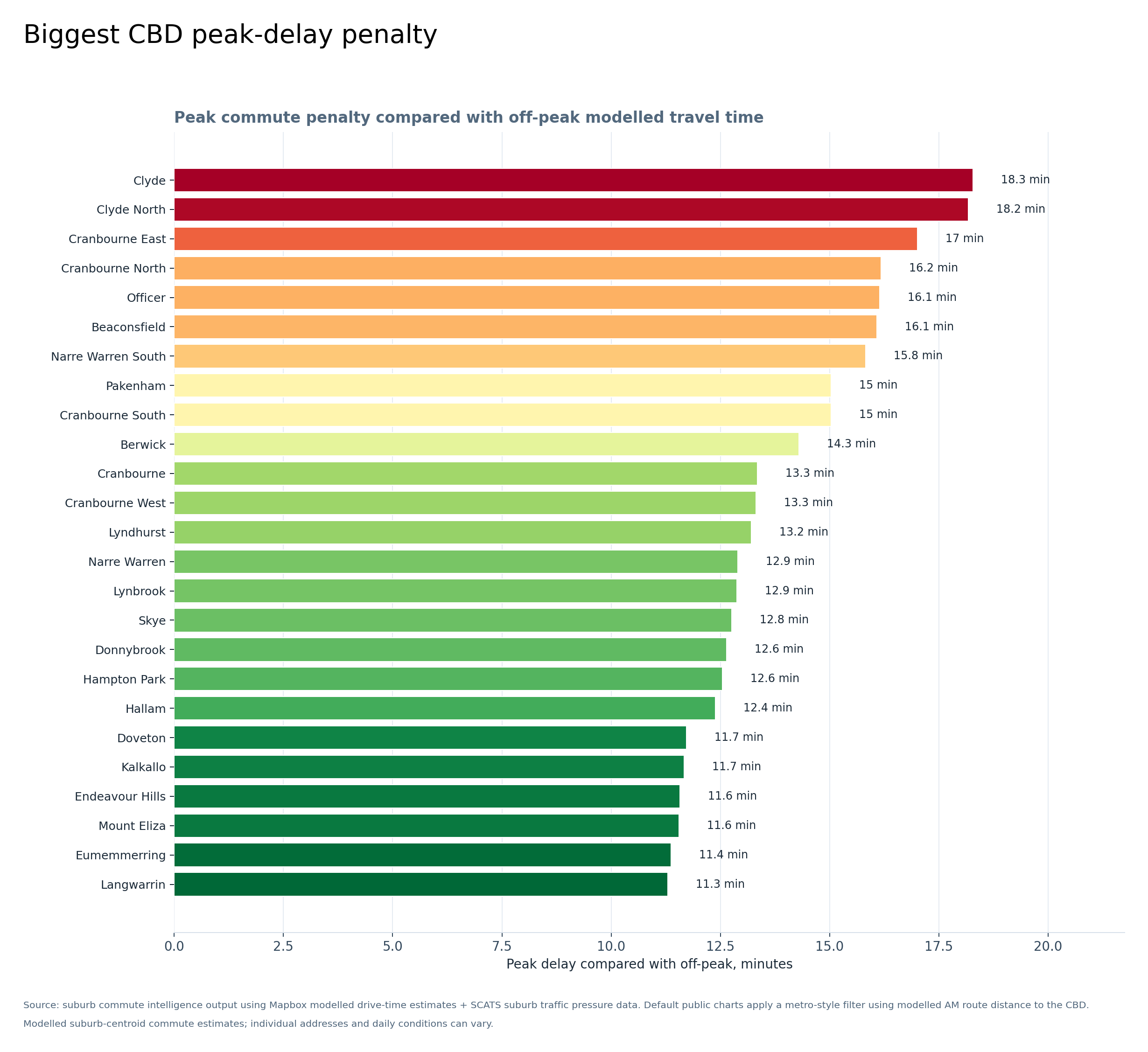
Graph 4 — Biggest CBD peak-delay penalty
This graph compares peak commute time with off-peak travel time. The higher the suburb appears, the more peak hour adds to the trip.
Clyde, Clyde North, Cranbourne East, Cranbourne North, Officer, Beaconsfield and Narre Warren South stand out as areas where peak conditions add substantial time.
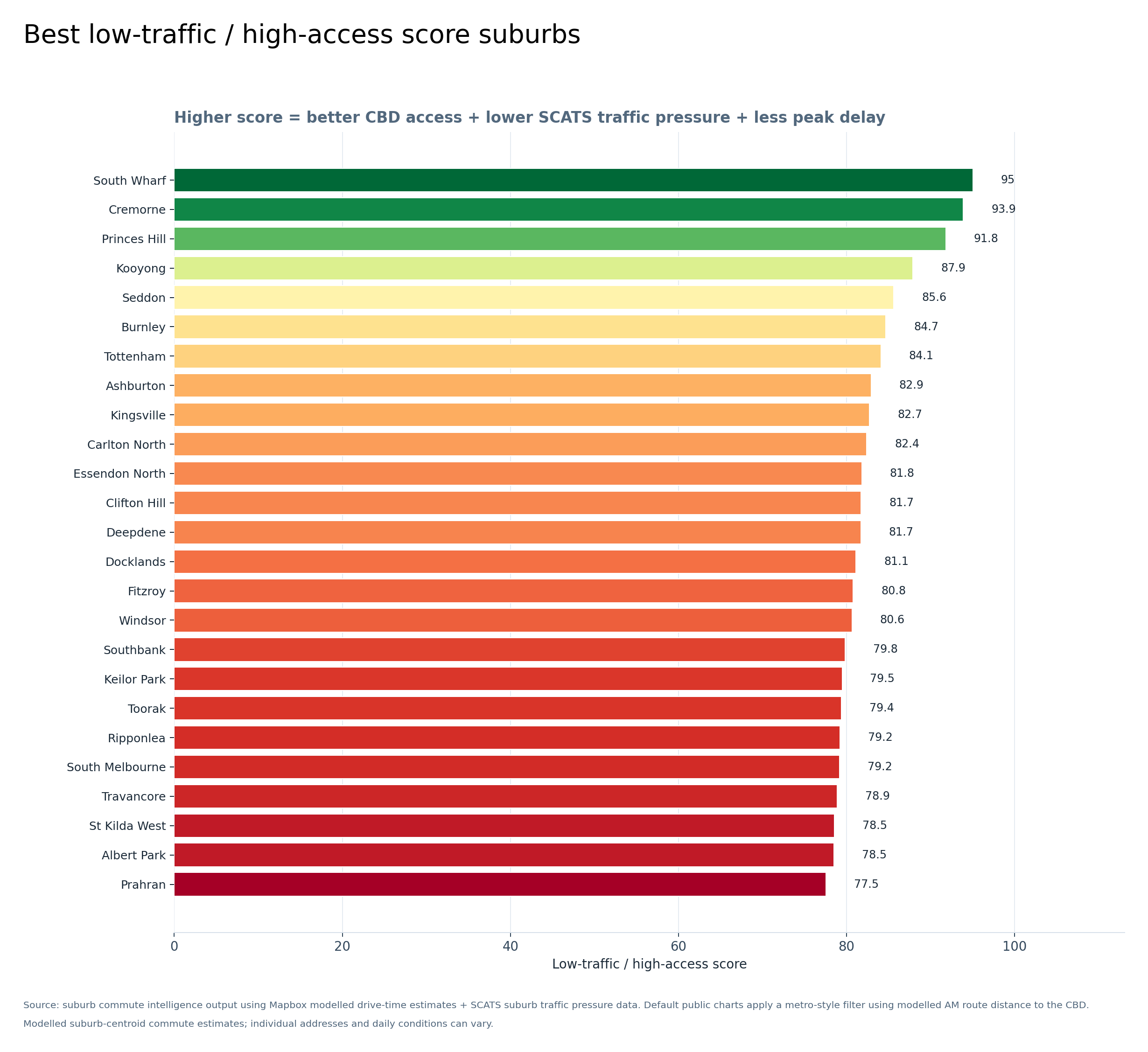
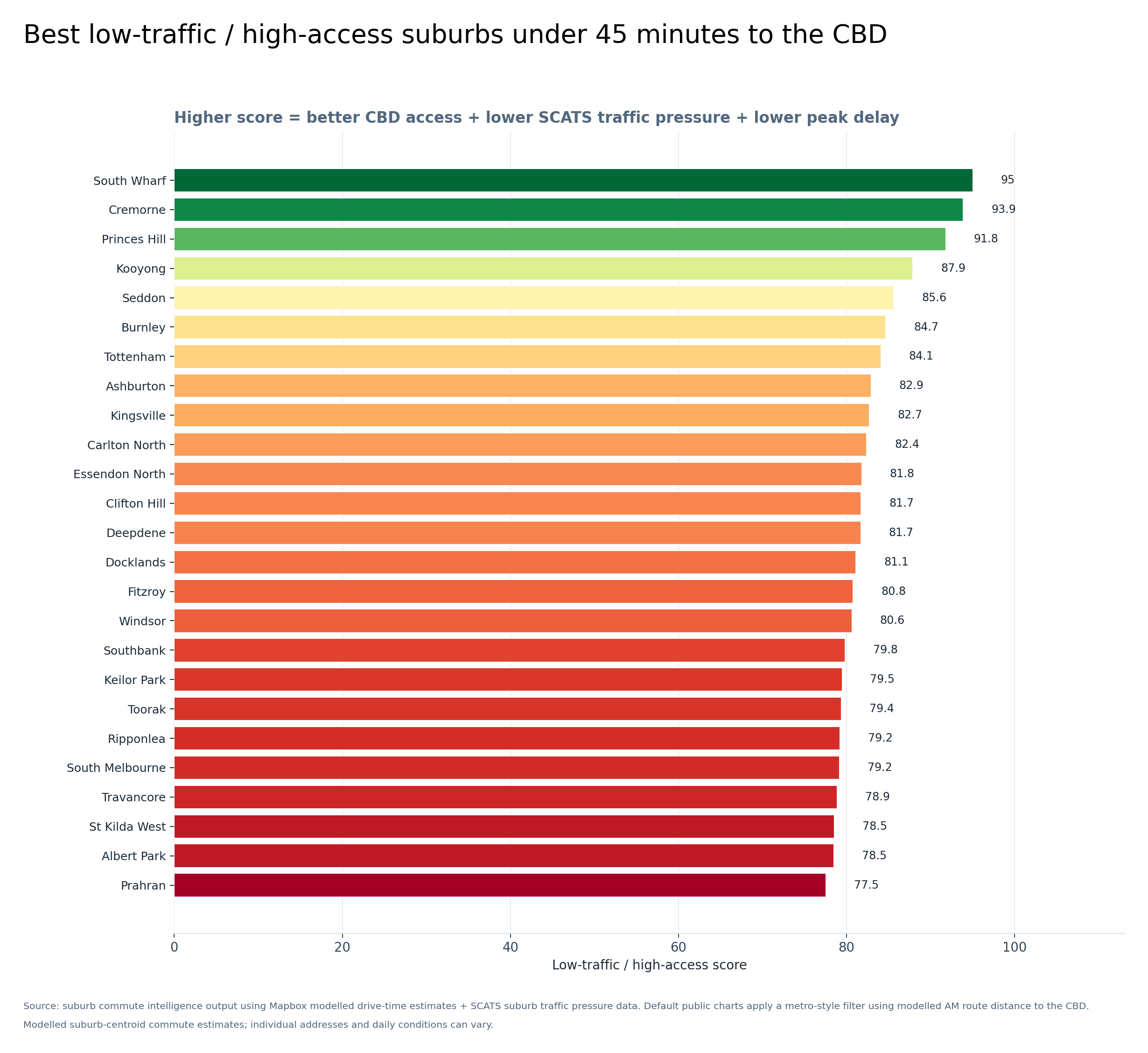
Graph 5 — Best low-traffic / high-access score suburbs
This score combines better CBD access, lower SCATS suburb traffic pressure and lower peak delay. South Wharf, Cremorne, Princes Hill, Kooyong, Seddon, Burnley, Tottenham, Ashburton, Kingsville and Carlton North perform well on this combined score.
This does not mean a suburb is silent or free of traffic; it means it scores well on this particular low-traffic / high-access comparison.
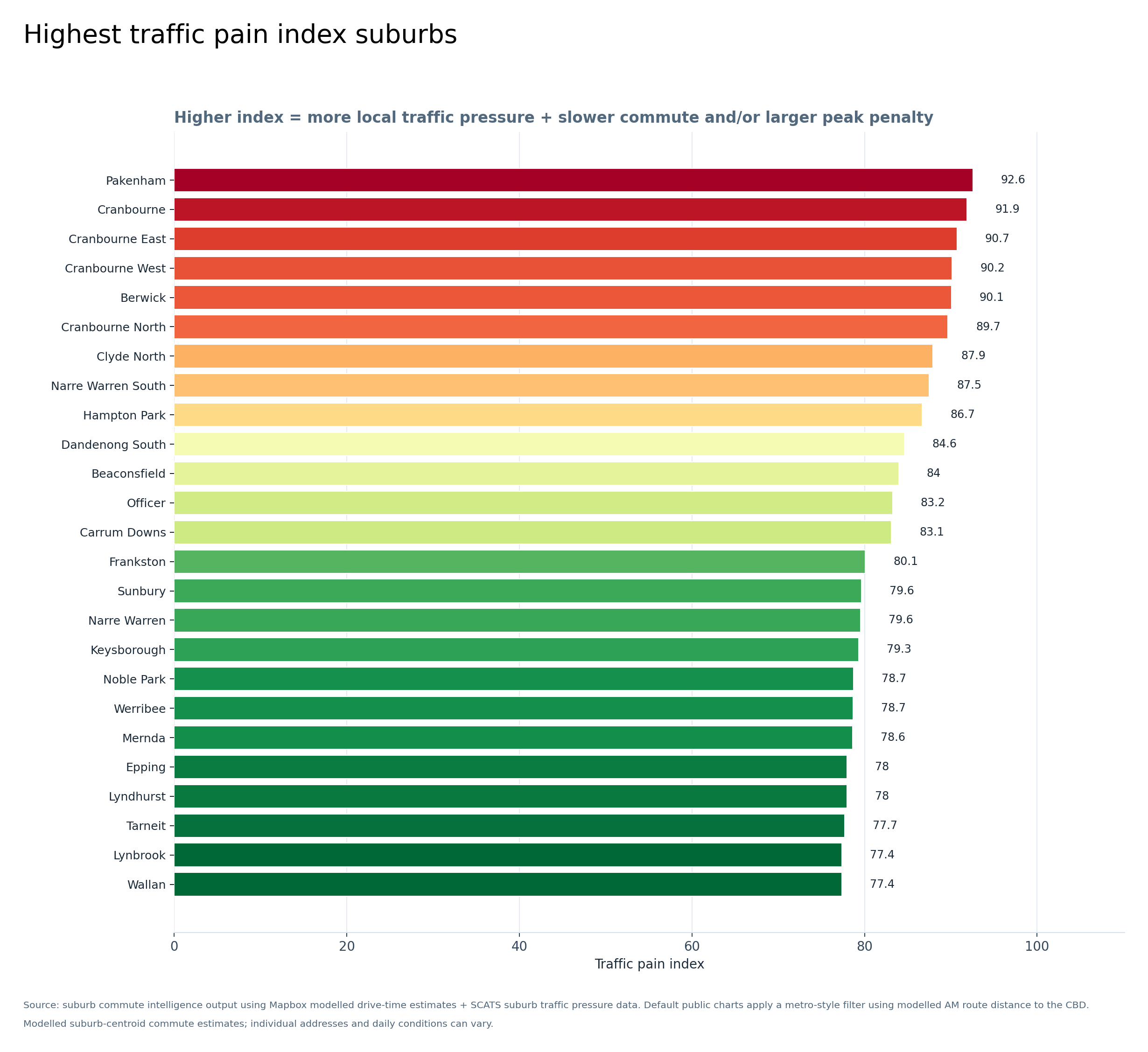
Graph 6 — Highest traffic pain index suburbs
This is one of the most important graphs. The traffic pain index combines local traffic pressure, slower CBD commute time and/or larger peak delay. Pakenham, Cranbourne, Cranbourne East, Cranbourne West, Berwick, Cranbourne North, Clyde North and Narre Warren South are all near the top.
The south-east growth corridor is very clearly visible here.
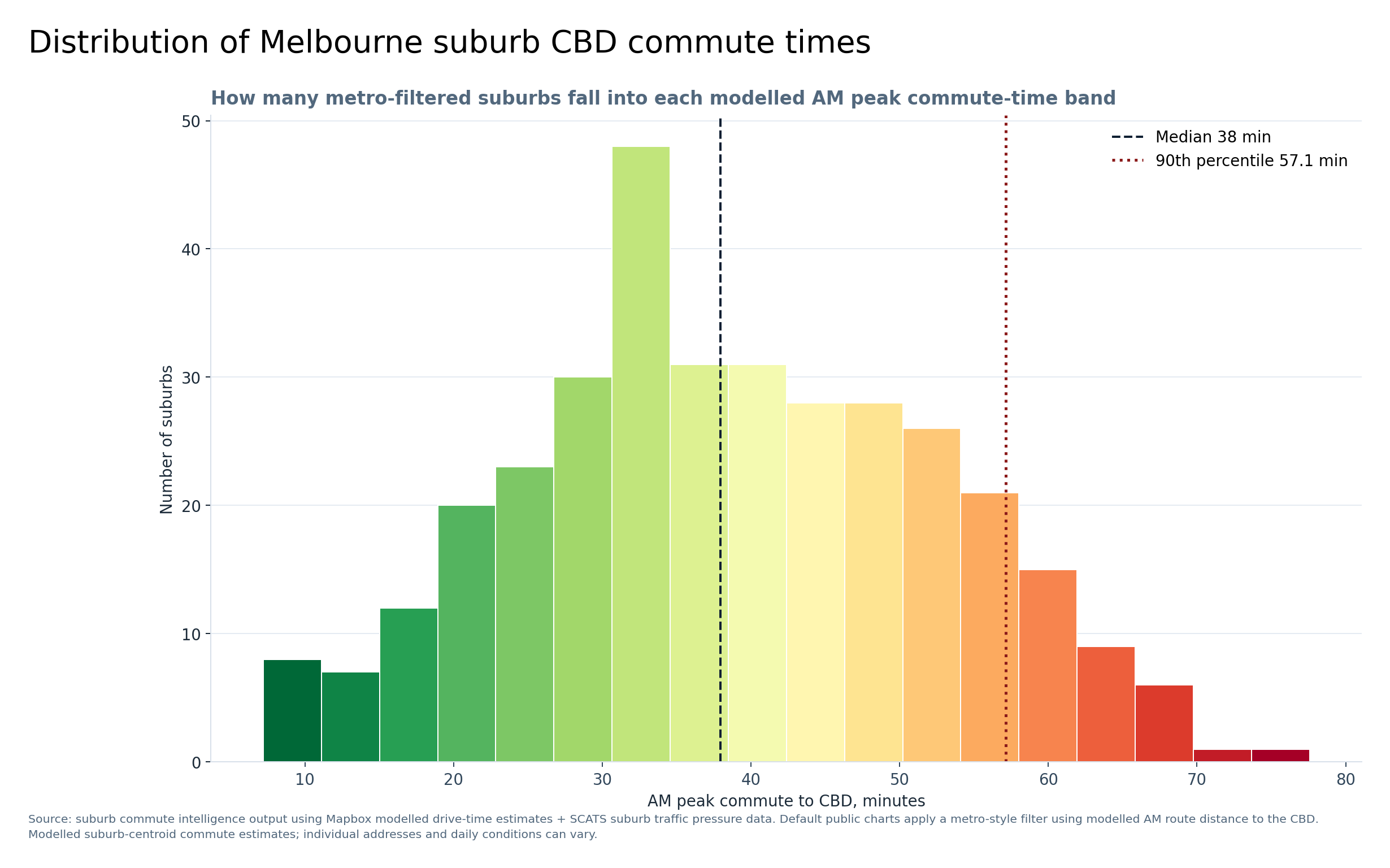
Graph 7 — Distribution of Melbourne suburb CBD commute times
This graph shows the overall spread of modelled AM peak CBD commute times across the metro-filtered suburbs. The median is about 38 minutes, while the 90th percentile is about 57 minutes.
Rather than only looking at individual suburbs, this shows the overall shape of Melbourne’s CBD commute burden.
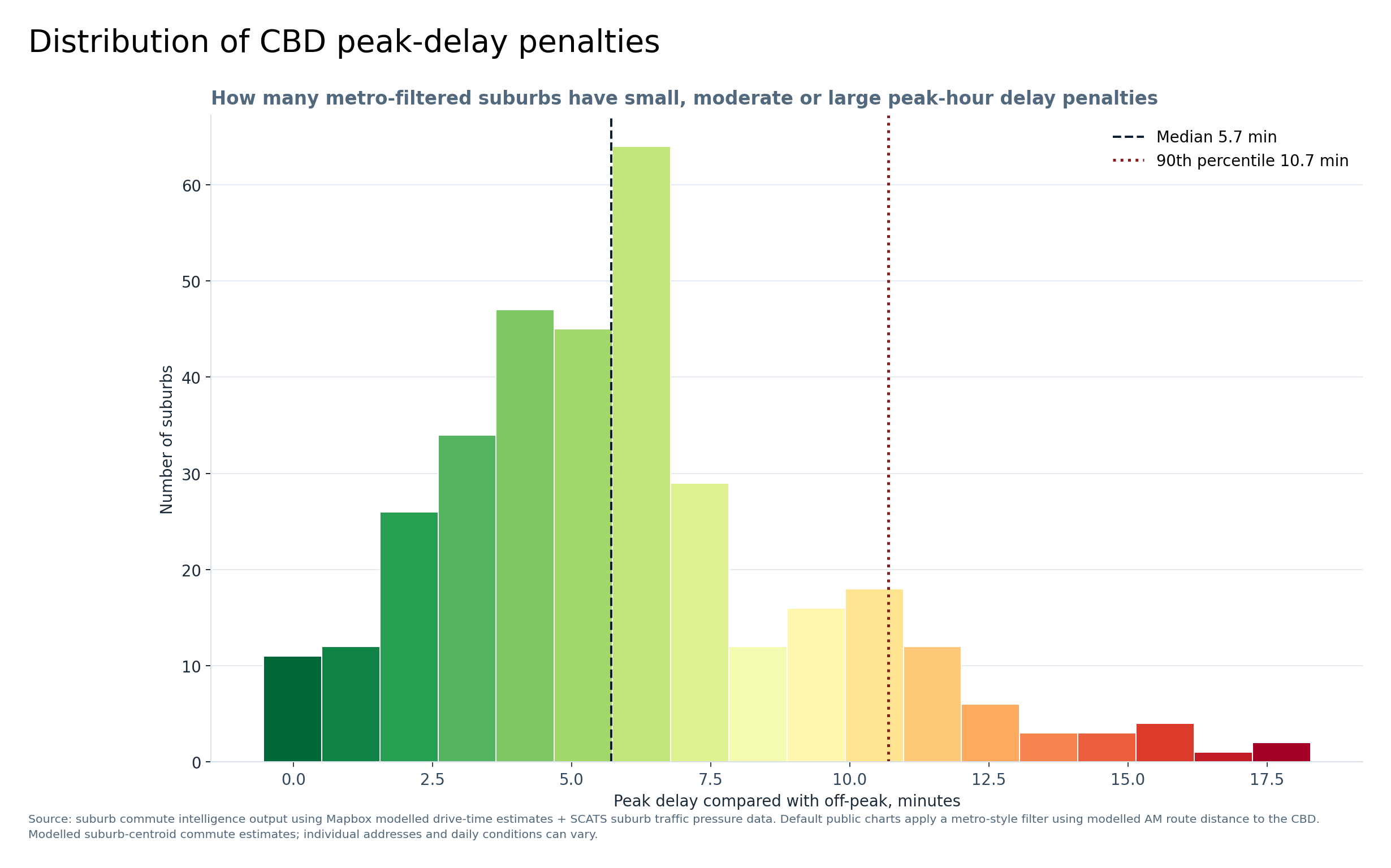
Graph 8 — Distribution of CBD peak-delay penalties
This graph shows how much extra time peak hour adds compared with off-peak travel. The median peak-delay penalty is about 5.7 minutes, while the 90th percentile is about 10.7 minutes.
Some suburbs are only slightly affected by peak hour, while others face a much larger delay penalty.
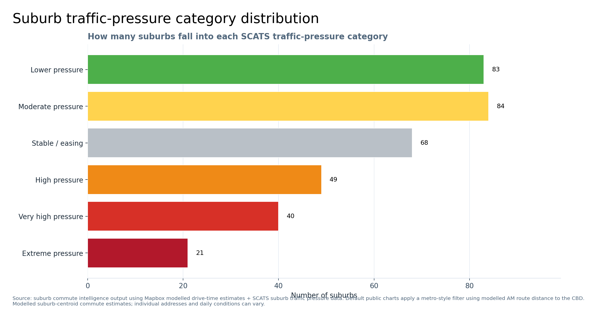
Graph 9 — Suburb traffic-pressure category distribution
This graph counts how many suburbs fall into each SCATS traffic-pressure category. It shows that Melbourne is not evenly loaded: some suburbs sit in lower or moderate traffic-pressure bands, while a smaller but important group falls into high, very high and extreme traffic-pressure categories.
This is based on cleaned SCATS suburb traffic-pressure data.
Graph 10 — Best low-traffic / high-access suburbs under 45 minutes to the CBD
This is a more practical version of the low-traffic / high-access score because it only includes suburbs under 45 minutes to the CBD in the modelled AM peak estimate.
Useful for people asking: where could I live with decent CBD access but less traffic pressure?
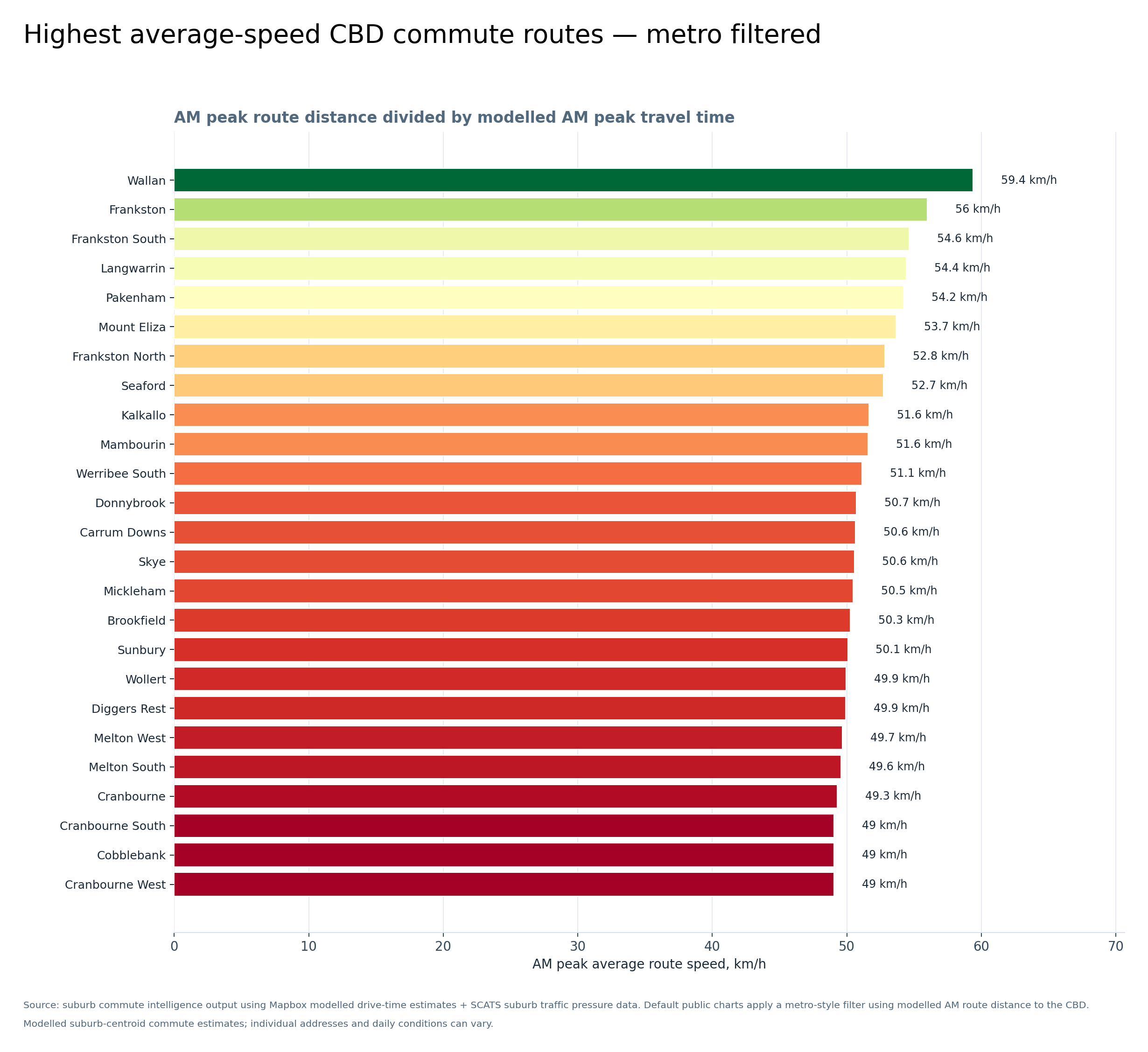
Graph 11 — Highest average-speed CBD commute routes, metro filtered
This graph shows AM peak route distance divided by modelled AM peak travel time. Outer suburbs with more freeway or arterial-style access can sometimes show higher average speeds, even if the total trip is longer.
This is not saying these are the best commutes — it shows route efficiency, not total convenience.
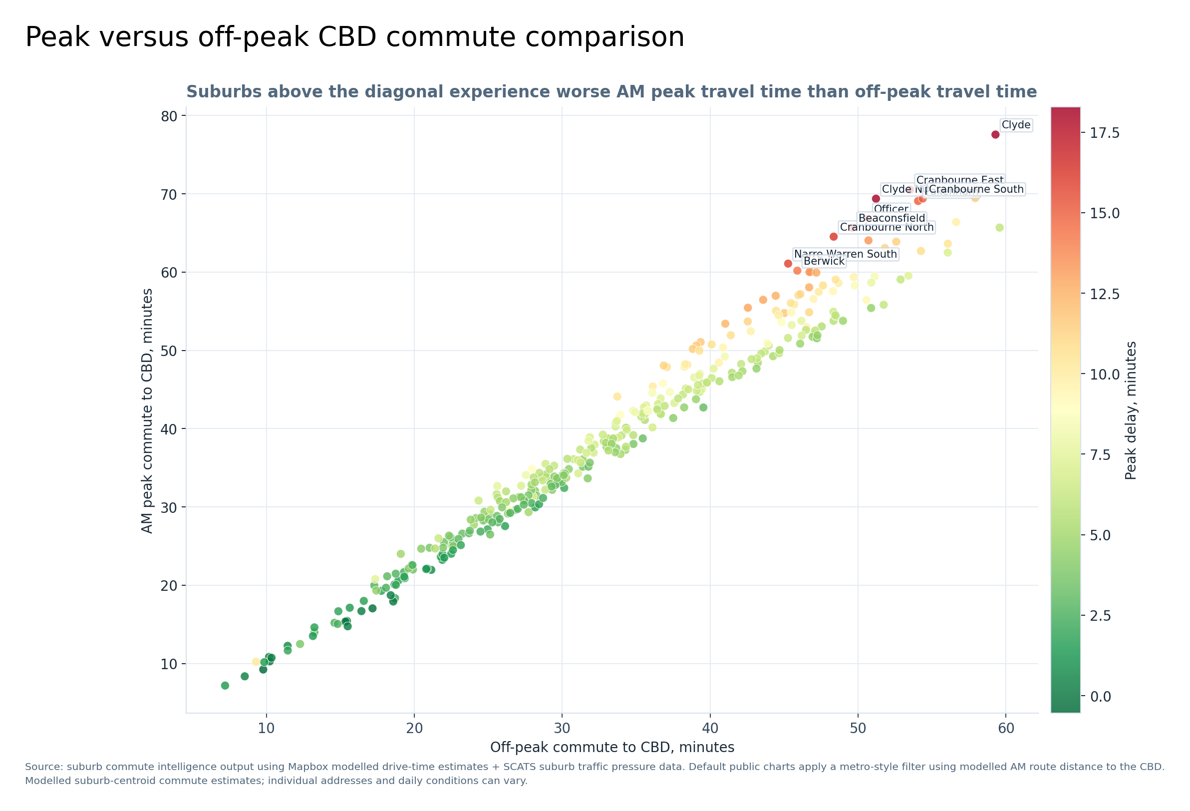
Graph 12 — Peak versus off-peak CBD commute comparison
Each dot is a suburb. The further above the diagonal a suburb sits, the worse the AM peak commute is compared with off-peak.
The labelled suburbs near the upper right are where longer commute times and larger peak delays combine.
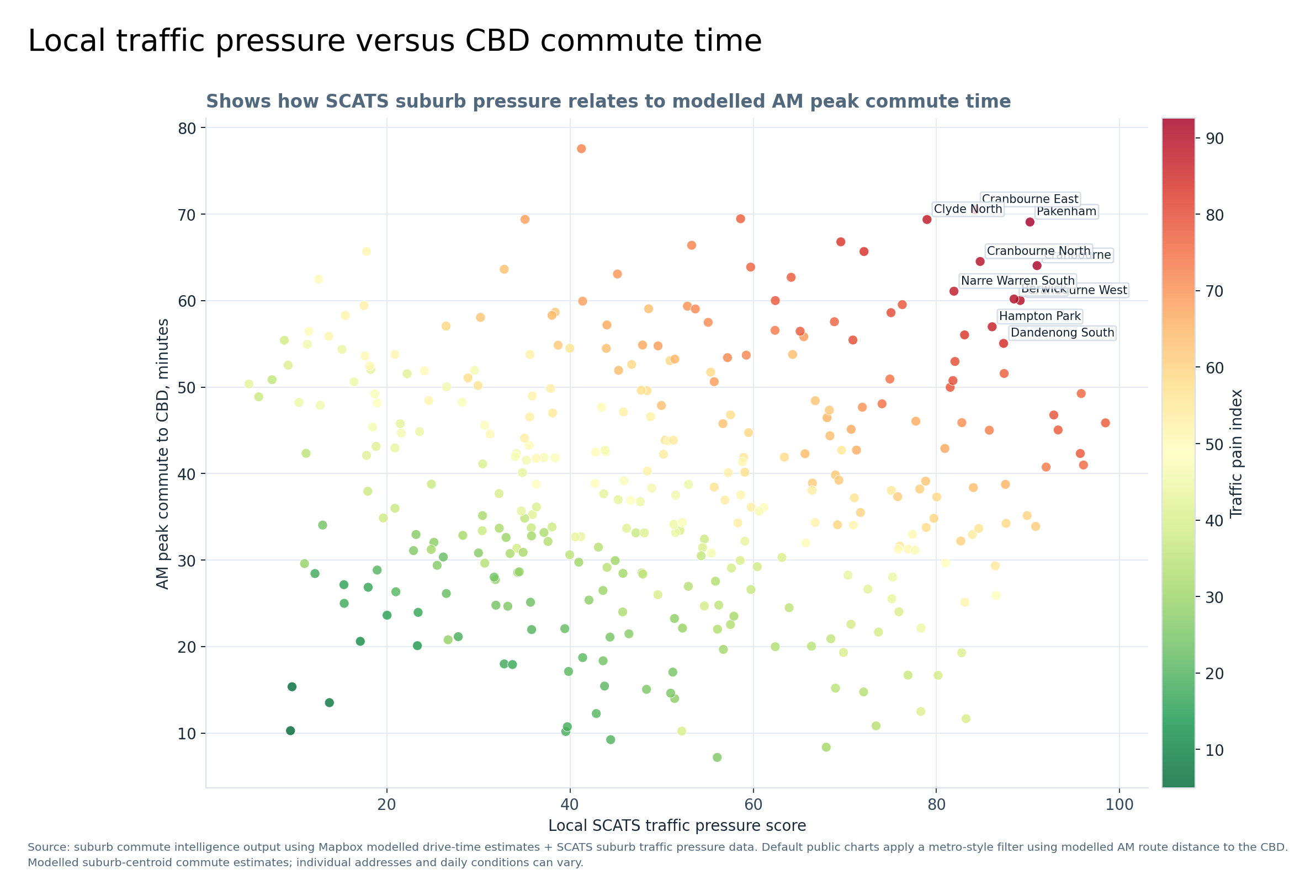
Graph 13 — Local traffic pressure versus CBD commute time
This graph combines two different things: local SCATS suburb traffic pressure and modelled AM peak CBD commute time. The most interesting suburbs are toward the upper right, where high local traffic pressure and longer CBD commute times combine.
That is where traffic pain becomes more than just distance from the city.
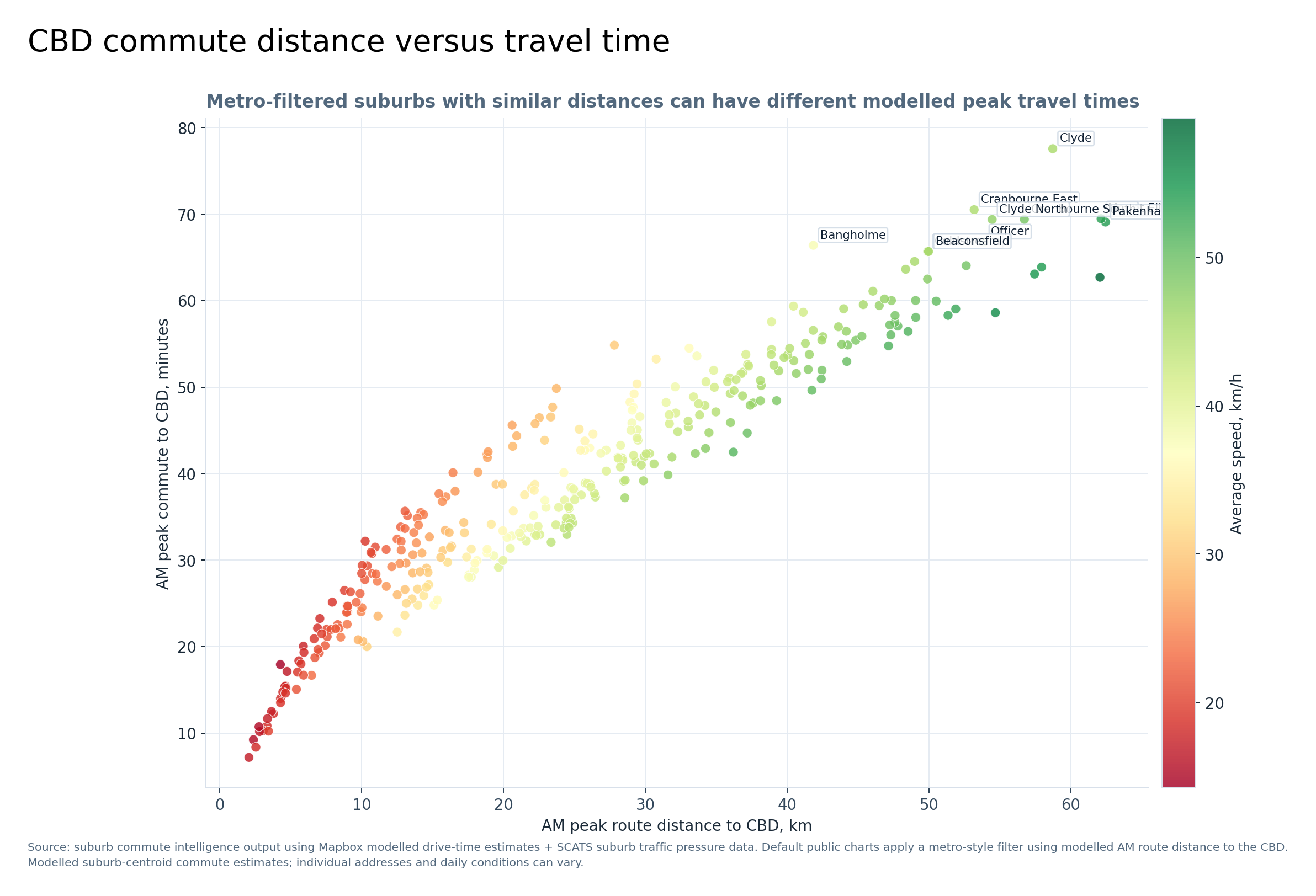
Graph 14 — CBD commute distance versus travel time
This graph shows the relationship between route distance and modelled AM peak travel time. Distance matters, but it is not the whole story.
Some suburbs at similar distances can have noticeably different travel times depending on road access, congestion, route structure and peak-hour delay.
Melbourne’s Top 100 Busiest Traffic Suburbs
A ranked suburb-level view of Melbourne traffic pressure, built from cleaned SCATS vehicle movement data.
This section sits alongside the suburb profile search above: search for your suburb, then use this Top 100 table
to see how it compares against Melbourne’s busiest traffic locations.
100suburbs ranked in this table
328,222,558,357vehicle movements across the Top 100
2,431SCATS sites counted across these suburbs
Melbourne#1 suburb · 19,588,962,503 movements
Ranking basis: total vehicle movements aggregated by geocoded suburb. This is a traffic-load ranking,
not a population ranking. The busiest-site column identifies the highest-volume SCATS site contributing
to each suburb’s total.
HTML profile links use the existing suburbtraffic/ report folder; PDF links use suburbtraffic/pdfs/ and the same suburb-profile naming convention.
Melbourne Suburbs Where Traffic Has Gotten Worse Since 2014
A suburb-level growth view built by joining monthly SCATS site totals to the suburb lookup layer.
The headline comparison uses full-year 2014 vs 2025. The 2026 figure is shown only as
Jan–Apr year-to-date monitoring, not as a full-year comparison.
Loading…Melbourne metro suburbs analysed
Loading…biggest absolute increase
Loading…extra movements, 2014 to 2025
Loading…highest same-site percentage growth
The absolute-growth table answers: where has the total measured traffic burden grown most?
The same-site table is more conservative because it only compares SCATS sites present in both 2014 and 2025.
Important caveat: raw suburb growth can be affected by new SCATS sites being added over time.
Use the same-site table when you want the cleaner like-for-like comparison.
Loading suburb traffic growth data…
CSV source expected at:
downloads/melbourne_metro_suburb_traffic_growth_2014_2025_with_2026_ytd.csv.
HTML profile links use suburbtraffic/; PDF links use suburbtraffic/pdfs/.
Melbourne Traffic Pressure Index by Suburb
A combined suburb ranking showing where traffic is already heavy and still getting worse.
The index blends 2025 traffic burden, absolute growth from 2014 to 2025,
and same-site growth to identify the suburbs under the strongest measured traffic pressure.
Loading…Melbourne metro suburbs scored
Loading…#1 pressure suburb
Loading…highest pressure score
Loading…suburbs in extreme pressure category
Why this matters
The busiest-suburbs table shows current traffic load. The growth table shows change over time.
This index combines both to identify where traffic is already heavy and still worsening.
Index formula
45% current 2025 traffic burden percentile + 35% absolute growth percentile +
20% same-site growth percentile, adjusted by a confidence multiplier.
Interpretation note: this is a ranking index, not a government congestion model.
It is designed to surface public-interest suburb pressure signals from the cleaned SCATS movement layer.
Rank
Suburb
Score
Category / confidence
2025 movements
Growth since 2014
% growth
Same-site growth
Sites
2026 YTD
Links
Loading Melbourne Traffic Pressure Index…
CSV source expected at:
downloads/melbourne_traffic_pressure_index_by_suburb.csv.
HTML profile links use suburbtraffic/; PDF links use suburbtraffic/pdfs/.
Important Intersection Intelligence
The older “Top 50” concept has been consolidated into the richer intersection intelligence already present on the page. Importance is now assessed using multiple lenses: cumulative movement, busiest-site ranking, Top 20 mapping, full SCATS network coverage, corridor dominance, site-month volatility and OOH opportunity value.
New behavioural layer: the completed time-bin run does more than identify the busiest and quietest 15-minute intervals. It now allows the page to explain how Melbourne accumulates traffic during the day, how long the network stays near capacity, how sharply it ramps up and drops off, and whether peak demand is scattered or tightly concentrated.
The key finding is that Melbourne is not merely a short “rush-hour” city. It behaves like a sustained high-volume plateau system with a concentrated afternoon pressure spike embedded inside it.
Peak pressure: 17:15Quiet baseline: 03:00>70% of peak for 11.2 hoursMorning ramp: 5.3×Top 10 bins: 15:15–17:30
50% of Daily Traffic Reached By
13:45
75% of Daily Traffic Reached By
17:15
Traffic Completed by 5PM
73.8%
Traffic Completed by 7PM
86.3%
Afternoon vs Morning Peak
1.18×
Top 10 Bin Cluster Span
2.2 hrs
1. Melbourne Uses Most of Its Daily Traffic Before Evening
By 5PM, approximately 73.8% of daily traffic has already occurred. By 7PM, the figure rises to about 86.3%.
2. The Day Is Plateau-Driven, Not Just Peak-Driven
The network remains above 70% of peak for about 11.2 hours, above 80% for 8.0 hours, and above 90% for 3.2 hours.
3. Afternoon Pressure Is Structurally Higher
The afternoon pressure window is about 1.18× the morning-window peak, showing that the PM period carries stronger sustained load than the morning build-up.
4. The Busiest Intervals Are Tightly Clustered
The top 10 busiest 15-minute intervals cluster between 15:15 and 17:30, making the strongest exposure period highly concentrated and commercially useful.
Behavioural Analytics Charts
Cumulative Daily Traffic Curve
Shows how quickly Melbourne accumulates its daily road-network activity and when major cumulative thresholds are reached.
Commercial interpretation: this gives OOH and media planners a highly specific high-exposure window, rather than a generic “PM peak” label.
Story interpretation: Melbourne’s signalized-road activity is best described as a long high-volume operating plateau with an embedded afternoon pressure spike. The city does not simply “peak”; it stays busy for much of the business day, then concentrates its strongest 15-minute intervals into a narrow late-afternoon window.
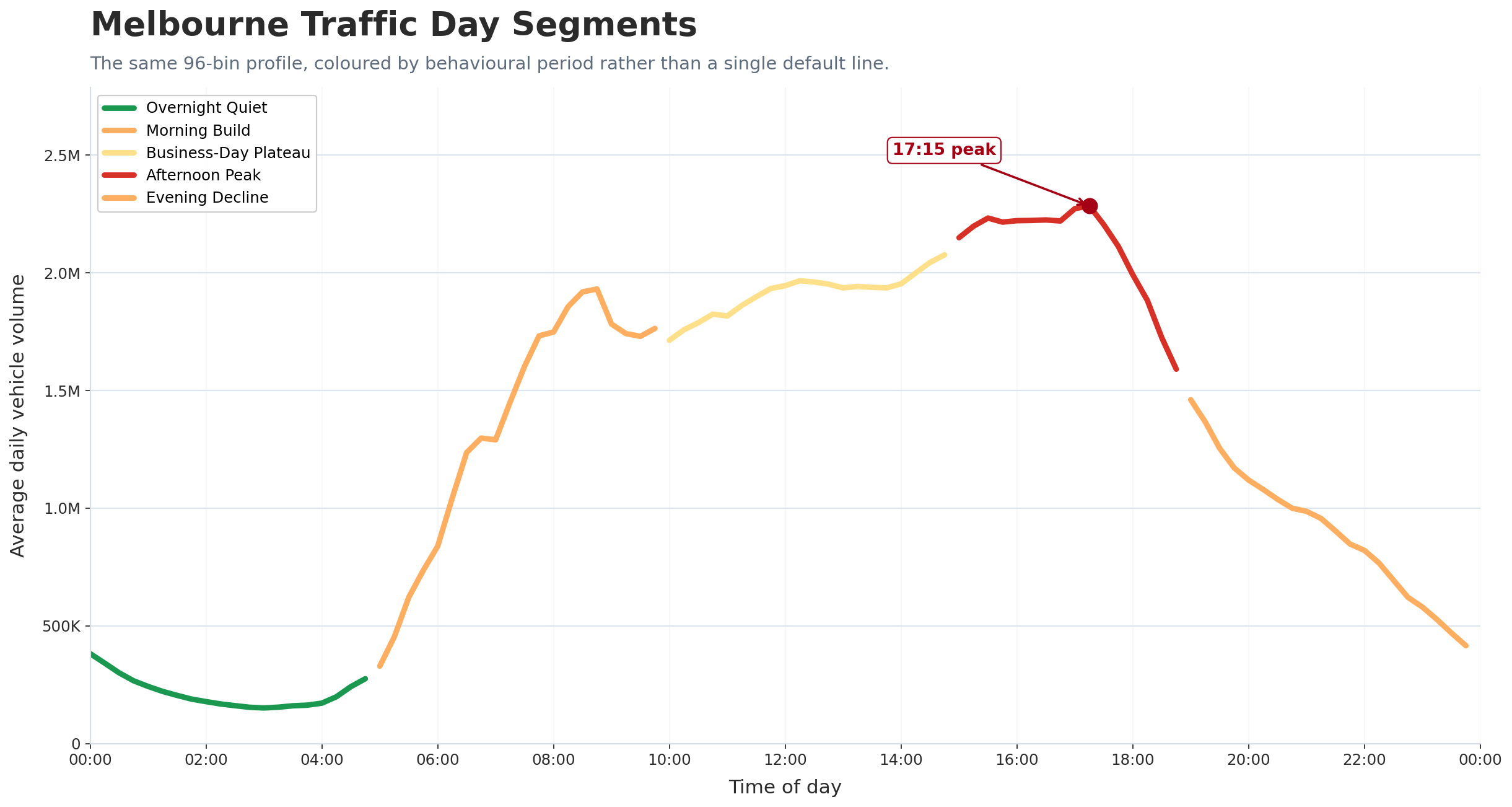
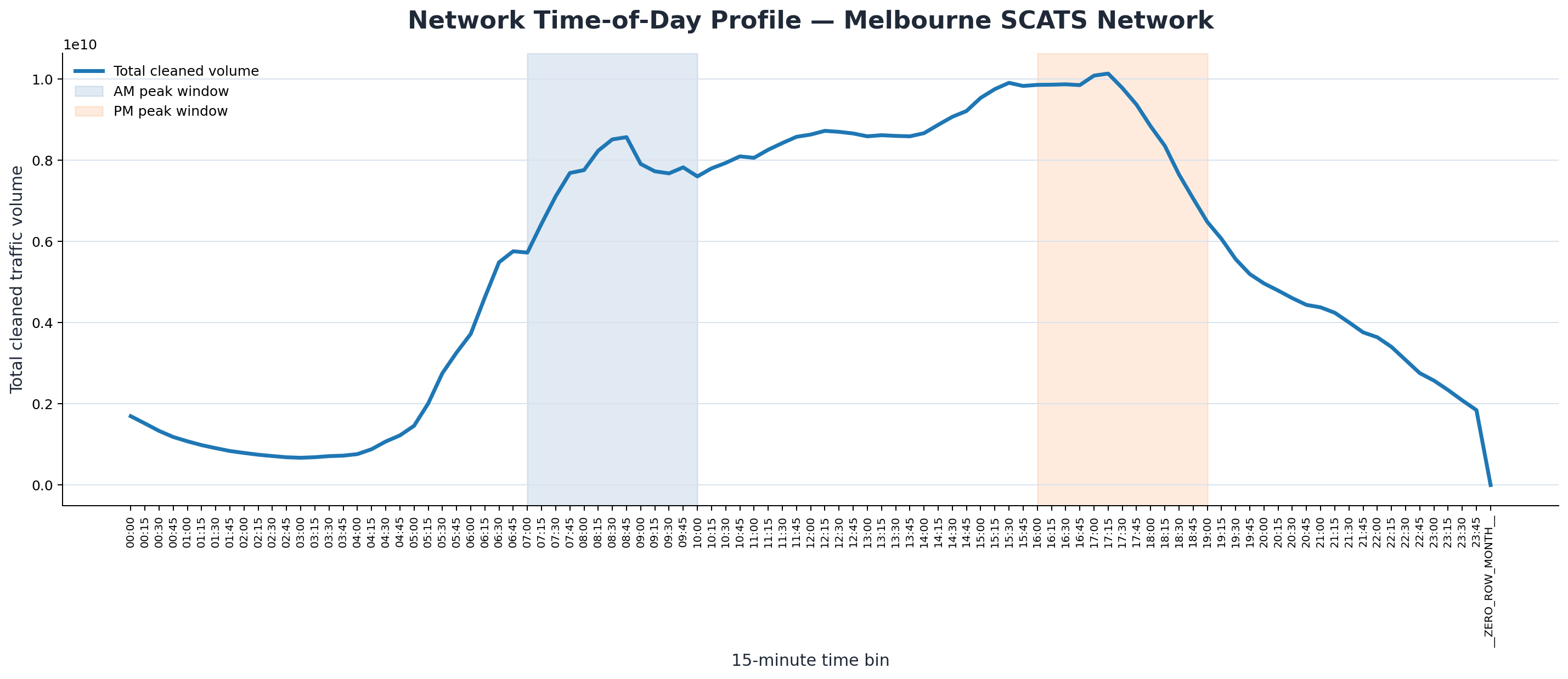
Production Time-of-Day Traffic Profile — When Melbourne Moves
Completed 96-bin daily rhythm model
The completed time-bin workflow now gives the page a full 15-minute profile of Melbourne's signalized road network across the archive.
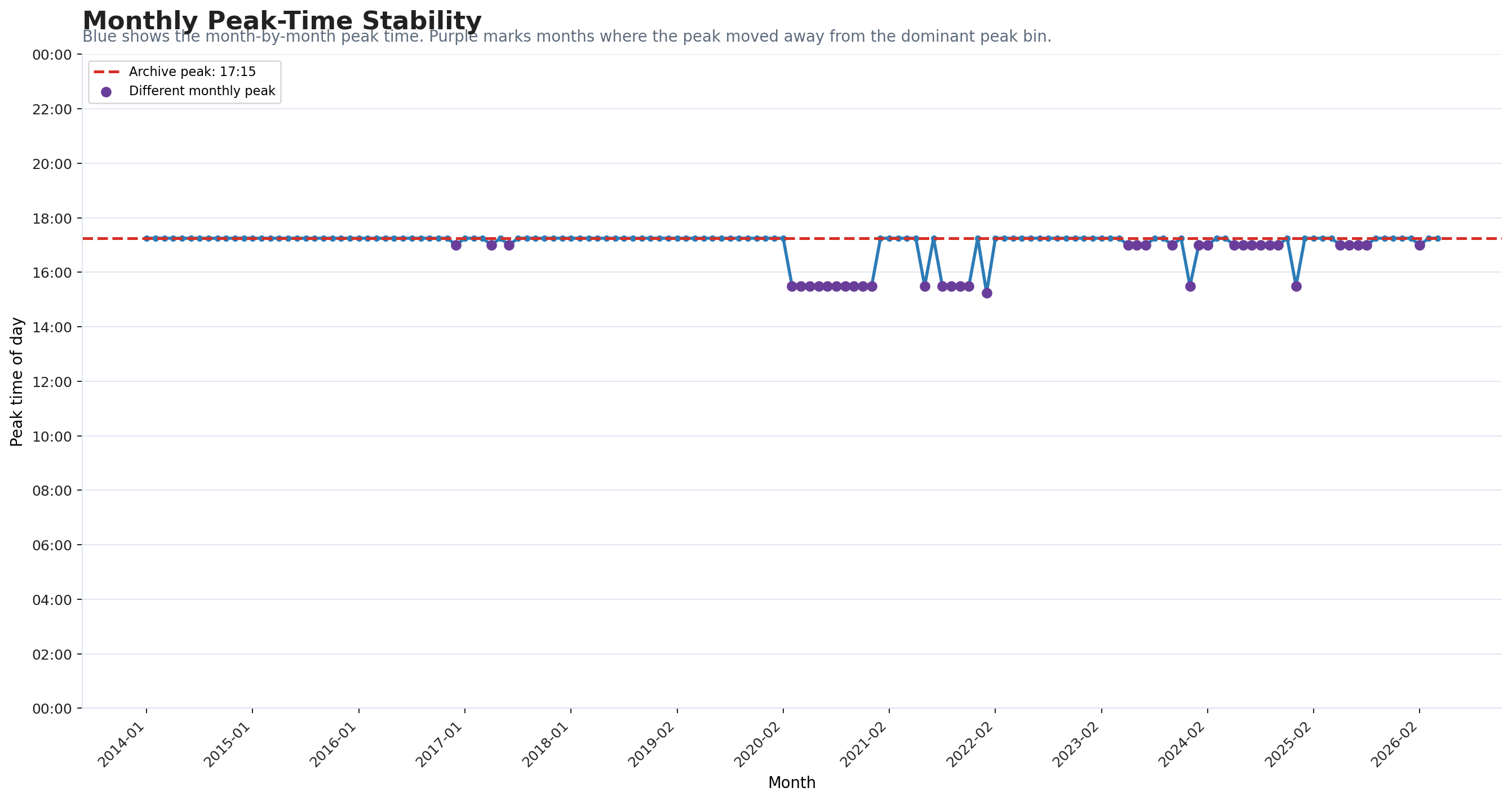
The strongest average daily interval is 17:15, while the quietest interval is 03:00.
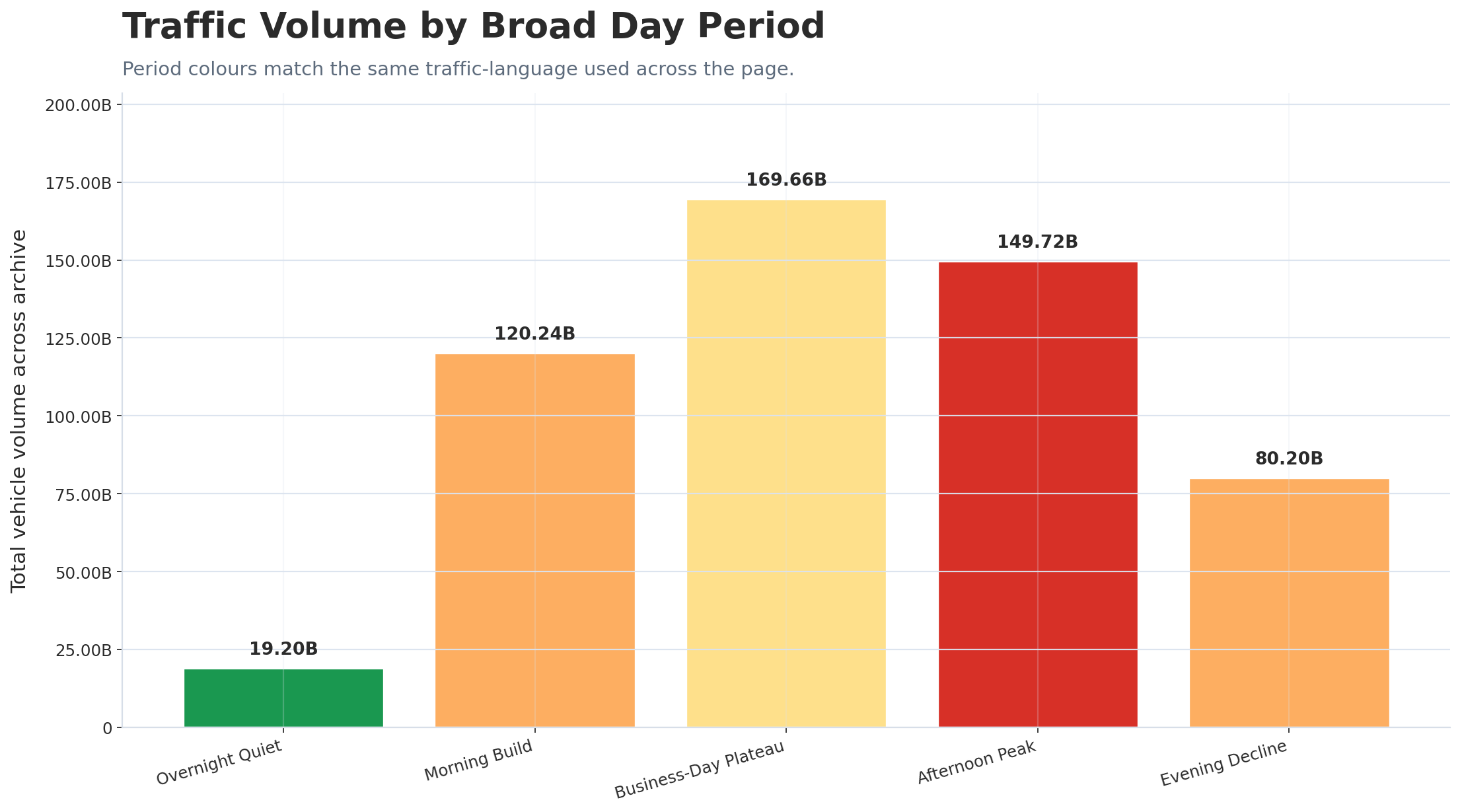
This turns the archive from a set of totals into a readable daily movement pattern: overnight quiet, morning build, business-day plateau, afternoon peak, and evening decline.
Public-facing interpretation: Melbourne does not simply have a generic “afternoon peak”.
In this archive, the strongest network-wide 15-minute point is precisely 5:15pm to 5:30pm.
The quietest point is around 3:00am to 3:15am. This is a simple, quotable finding for journalists and a direct exposure-timing signal for OOH media.
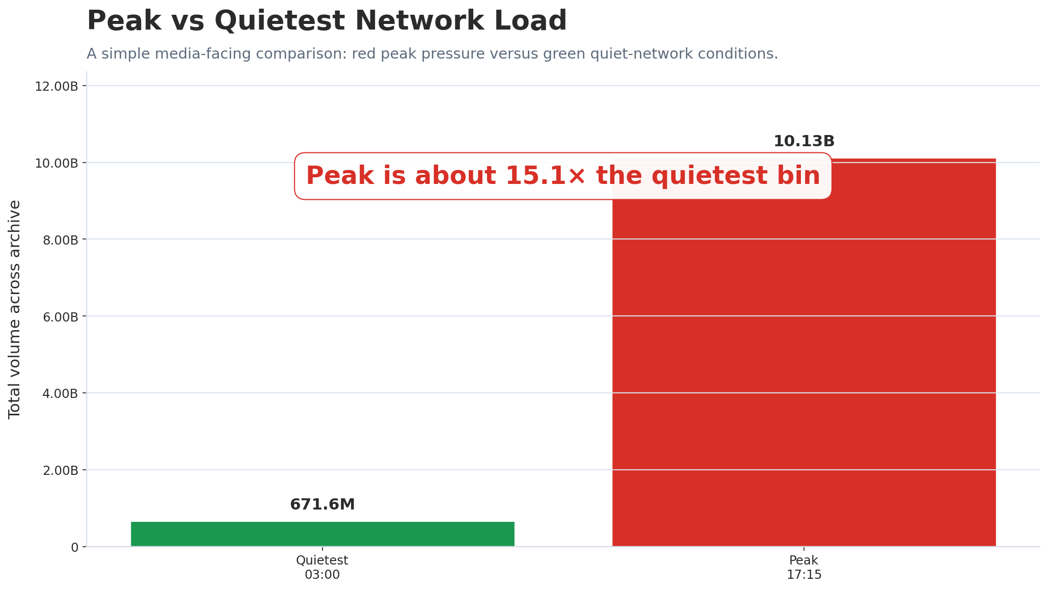
Main Chart — Melbourne Traffic Daily Rhythm
The headline chart showing the full 24-hour movement curve, with the 17:15 peak and 03:00 quietest point annotated.
How strong is the daily swing? The peak bin is about 15.1 times the quietest bin.
Is the PM peak real or vague? It is measurable, narrow, and strongly clustered around late afternoon.
Why this matters
Journalists get a precise headline rather than a vague “rush hour” claim.
OOH media gets an exposure-timing layer for audience-value analysis.
Transport analysts get a city-wide behavioural rhythm that can be compared with incidents, school terms, holidays, weather, and future infrastructure changes.
The completed day-of-week profile turns Melbourne's SCATS archive into a weekly behavioural model of the city. Across the cleaned and deduplicated period from 1 January 2014 to 7 April 2026, the script processed 148 / 148 months, produced 1,029 analytical rows, and completed in approximately 32.5 hours. The result is a clear weekly movement signature: traffic builds from Monday through the working week, reaches maximum intensity on Friday, then falls sharply into the Saturday and Sunday rest state.
Headline interpretation: Melbourne's strongest average day is Friday at approximately 133.0 million detected daily movements. The weakest is Sunday at approximately 97.3 million. That means Friday operates around 36.7% stronger than Sunday, while Friday is around 11.4% stronger than Monday.
This section is one of the most human-readable layers of the SCATS project. It does not merely count vehicles; it shows the rhythm of the working week, the weekend collapse, COVID-era behavioural disruption, recovery, seasonality, and the persistent structural weakness of Mondays relative to the later working week.
The completed profile shows a smooth, intuitive pattern: Monday starts lower, Tuesday and Wednesday strengthen, Thursday nears saturation, Friday peaks, and the weekend drops sharply.
2. Friday is the structural peak
Friday is not merely a noisy outlier. It remains the strongest day across the full completed archive, combining commuting, freight, retail, hospitality, nightlife, and late-week discretionary movement.
3. Sunday is a true rest state
Sunday sits far below Friday and below Saturday, giving the city a clear weekly decompression signature that is highly visible in both bar charts and heatmaps.
4. Monday weakness is persistent
Monday is consistently weaker than the Tuesday-to-Friday working week, suggesting a real behavioural structure rather than random month-to-month variation.
5. COVID changed the weekly shape
The era comparison charts show the COVID-shock period compressing the entire weekly curve downward, followed by a recovery/new-normal profile that rises above the pre-COVID average.
6. Weekends are more volatile
Saturday and Sunday show higher month-to-month volatility than most weekdays, consistent with discretionary travel, events, holidays, weather sensitivity, and pandemic disruption.
Headline Day-of-Week Charts
These charts show the core weekly movement signature: Friday peak, Sunday rest state, workweek build-up, and the long-term day-of-week heat structure.
Melbourne Weekly Traffic Heartbeat
The core weekly rhythm chart: Monday starts lower, the workweek builds steadily, Friday reaches maximum average daily movement, then the network drops into the weekend.
Simple headline: Melbourne builds toward Friday. The SCATS archive shows a clear weekly behavioural signature: the city intensifies through the workweek, peaks on Friday, and drops into a Sunday rest state.
Why it matters: this is useful for transport planning, OOH advertising, retail, events, freight, hospitality, journalism, and public understanding because it translates billions of detector observations into a familiar weekly rhythm.
Confirmed result:
Across the full cleaned Melbourne SCATS archive from 1 January 2014 to 7 April 2026, weekdays account for 404.9 billion detected movement events, while weekends account for 134.1 billion. That equals 75.13% weekday traffic and 24.87% weekend traffic across 539.0 billion total analysed movement events.
Behavioural interpretation: this section turns the SCATS archive from a pure volume count into a citywide behavioural model. It shows how much of Melbourne's movement economy is work-week driven, how resilient weekend traffic is, how the COVID disruption affected weekday and weekend patterns differently, and how strongly weekend daily intensity has recovered.
The key public-facing insight is simple: Melbourne is weekday-dominant, but not weekday-only. Even after normalising for the number of days, a typical weekend day still reaches around 82.7% of weekday daily traffic intensity.
Three quarters of all detected SCATS movement events occur on weekdays, confirming the ongoing importance of work-week commuting, freight, school, services, and business activity.
Weekends still contribute 134.1 billion detected movements. For retail, events, hospitality, tourism, and outdoor advertising, that is not a minor residual market.
3. Normalised weekend intensity is the surprise
After adjusting for weekday and weekend day counts, a typical weekend day reaches about 82.7% of weekday traffic intensity. Melbourne remains highly mobile outside the work week.
4. COVID altered the balance, then recovery lifted weekends
The rolling weekend-share and relative-intensity charts show a visible lockdown-era break, followed by a recovery period where weekend share trends higher than the pre-COVID baseline.
Weekday vs Weekend Dashboard Summary
A one-image overview of the entire weekday/weekend behavioural layer, suitable for media, internal briefings, and social sharing.
Best media headline: Melbourne's traffic economy is overwhelmingly weekday-driven, but weekends still carry 134.1 billion detected vehicle movement events and a typical weekend day still reaches 82.7% of weekday daily intensity.
How to read this section: blue represents weekday movement, orange represents weekend movement, the pale red background marks the COVID disruption window used in the charts, and the rolling-average line smooths month-to-month calendar noise so the underlying behavioural trend is easier to see.
Month-of-Year Seasonal Traffic Intelligence
The completed month-of-year workflow converts the full deduplicated Melbourne SCATS archive into a seasonal citywide movement profile.
Instead of asking only which individual month was largest, this section asks how Melbourne behaves across the calendar year: which months are structurally busiest, which months are quietest, how COVID reshaped seasonal behaviour, and where the strongest recovery-era traffic pressure now appears.
Busiest average month
FebruaryApproximately 128.5 million average daily vehicle movements.
Second strongest month
NovemberApproximately 128.3 million average daily vehicle movements.
Quietest month
JanuaryApproximately 114.4 million average daily vehicle movements.
Peak-to-trough gap
~14.1 million/dayThe February to January difference is large enough to be visible at whole-city scale.
Workflow runtime
34.3 hoursThe completed month-of-year process ran for 123,587 seconds across the full 2014–2026 archive.
February peakNovember peakJanuary holiday troughMarch highest cumulative monthRecovery era now above pre-COVID baseline34.3 hour seasonal workflow
Interpretation: February appears to represent Melbourne returning to full operational intensity after the January holiday slowdown: schools, workforces, freight, universities, retail activity and commuting patterns all re-enter the network at once. November is almost as strong, likely reflecting late-year economic and retail activity before the Christmas/New Year slowdown.
Melbourne seasonal traffic curve
The flagship calendar-year curve showing the average daily SCATS movement profile from January to December.
Cumulative cleaned traffic volume grouped by calendar month across the archive. March leads on total cumulative volume because it has more days and full-month coverage across more years.
Media angle: The finished seasonal profile supports a simple public story: Melbourne does not move evenly through the year. January is the holiday trough; February and November are the strongest operational months; March is the largest cumulative calendar-month bucket; and the post-COVID recovery era now visibly exceeds the pre-COVID baseline across much of the year.
Processing note: The completed month-of-year workflow reports 148 / 148 months processed, is_complete = true, a date range from 2014-01-01 to 2026-04-07, and one known zero-row month: 2018-12. The 2026 row should be interpreted as partial because the available archive ends on 2026-04-07.
This new CSV-only intelligence layer classifies Melbourne SCATS sites into behavioural road archetypes using the already-computed site rankings, site-month totals, growth, volatility, stability, spike behaviour, and mapped site metadata. It does not require another DuckDB pass. Instead, it turns the hundreds of hours of completed CSV outputs into a reusable classification model for transport, OOH media, journalism, and infrastructure analysis.
Why this matters: the page now moves beyond “which sites are busiest” into “what kind of traffic environment is this?” The V4 model separates metropolitan backbone corridors, reliable exposure corridors, mature urban arterials, balanced metropolitan sites, secondary connectors, rising growth corridors, volatile sites, disruption-sensitive sites, and stable local roads.
Classified SCATS Sites
4,758
Traffic Archetypes
11
Largest Class
Balanced Metropolitan Site
Largest Traffic Share
26.2%
Backbone Traffic Share
15.7%
New Index
Traffic Transformation
What the archetype model reveals
Balanced Metropolitan Sites are the largest road class by traffic share, carrying about 26.2% of analysed movement.
Mature Urban Arterials carry about 20.2%, showing that established non-freeway arterial structure is a major part of Melbourne movement.
Metropolitan Backbone corridors remain the pure OOH exposure leaders because they combine scale and stability.
High-Volume Volatile Corridors and Rising Growth Corridors dominate the Traffic Transformation Index because they combine change, volatility, growth, and scale.
The heatmap gives each archetype a behavioural fingerprint across scale, stability, volatility, growth, OOH exposure, transformation, and strategic importance.
One of the strongest system charts: it separates reliable backbone/exposure corridors from high-volume volatile corridors and local disruption-sensitive sites.
Method note: This is a derived intelligence layer, not a new raw-data query. It combines existing computed CSV outputs, including site rankings and site-month totals, to classify each SCATS site by traffic scale, stability, volatility, growth, spike behaviour, OOH exposure value, transformation intensity, and strategic importance.
Top 10 Behavioural Insights — What Melbourne Traffic Actually Does
This media-ready module turns the completed 15-minute time-bin analysis into clear, quotable findings. These are not just chart observations; they describe the operating personality of Melbourne’s signalized road network across a decade-plus archive.
1Melbourne’s strongest daily pressure point is 17:15
The archive identifies 17:15 as the busiest 15-minute interval, confirming that the strongest network load occurs in the late-afternoon commute rather than exactly on the hour.
2Melbourne is a plateau city, not just a peak-hour city
The network stays above 70% of peak for 11.2 hours, which means the city carries sustained high traffic for much of the day, not only during traditional commute windows.
3Half the day’s traffic has occurred by early afternoon
The cumulative curve shows that 50% of daily traffic is reached by about 13:45, revealing how much road activity is already complete before the evening peak begins.
4Nearly three-quarters of daily traffic is complete by 5PM
By 5PM, around 73.8% of the day’s traffic has already occurred. That makes the late afternoon not just a peak, but the final high-pressure phase of an already busy day.
5The top 10 busiest intervals cluster tightly in 2.2 hours
The strongest 15-minute bins are concentrated between 15:15 and 17:30. For media and OOH planning, that creates a precise high-exposure window rather than a vague “PM peak.”
6Afternoon pressure is structurally stronger than morning build-up
The afternoon peak window is about 1.18× the morning-window peak. Melbourne’s evening pressure is not simply the morning pattern repeated in reverse.
7Morning traffic ramps sharply from the overnight baseline
The morning ramp shows an approximate 5.3× increase from 05:00 to 08:00, capturing the network’s rapid transition from quiet baseline to commuter intensity.
8Evening traffic decays more gradually after peak
The 17:15 peak remains about 2.3× the 21:00 load, showing that pressure releases over several hours rather than disappearing immediately after the commute.
9The true quiet-network baseline is around 03:00
The archive identifies 03:00 as the quietest 15-minute interval. This gives the page a clear baseline for comparing how extreme daytime traffic load really is.
10Traffic value is time-dependent, not just location-dependent
The behavioural charts show that exposure quality changes dramatically by time of day. For commercial planning, a site’s value depends on when traffic passes as well as where it passes.
Media framing: Melbourne does not simply have “rush hour.” It operates as a long high-volume traffic plateau with a concentrated afternoon spike embedded inside it. That is a much more powerful and accurate story than a simple busiest-intersection ranking.
Top 10 Site-Month Insights — Named Sites and Hidden Network Nodes
This media-ready module turns the completed site-month charts into plain-English findings for journalists, advertisers, planners, and public readers.
Melbourne traffic has grown steadily over 12 years. Despite short-term disruptions, total network volume shows a clear long-term upward trend.
COVID caused the largest visible traffic collapse in the archive. The network monthly chart shows a dramatic 2020 drop followed by staged recovery.
Traffic has exceeded pre-COVID levels. By 2023–2025, Melbourne traffic recovered and pushed above earlier highs.
A small number of locations dominate the network. Sites such as Princes near Canning and Eastern Freeway / Hoddle carry enormous cumulative volume.
Growth is concentrated in specific corridors. The fastest-growing site-month outputs point to structural changes in how Melbourne moves.
Some of the most volatile records are network nodes, not named intersections. This exposes hidden traffic-control infrastructure in the SCATS network.
Traffic patterns are strongly seasonal. The heatmap shows annual rhythms, quieter periods, and stronger high-volume months.
Location value changes over time. A site’s importance is not only its total volume but how its monthly pattern changes across the archive.
Melbourne is thousands of micro-systems. The overall network can look stable while individual sites and nodes behave very differently.
The project now combines scale with human meaning. Friendly names, ranked sites, and network-node labels turn 539B movement events into a readable model of the city.
Media framing: This analysis captures both named signalised intersections and underlying SCATS network nodes, giving a broader picture of Melbourne traffic behaviour than a simple intersection ranking.
Site-Month Traffic Intelligence — Named Sites, Network Nodes, Growth and Volatility
Completed V5.2 site-month layer:
This module uses 595,054 site-month rows across 4,758 SCATS sites and joins the result to the SCATS metadata audit file so charts display friendly site names where available. Where no public friendly name exists, the chart labels the SCATS ID as a network node.
Note on “network node” labels: Some SCATS IDs are not listed in the public signalised-intersection register and do not have a friendly site name. These may represent detector stations, ramp meters, virtual/internal control points, or other SCATS network elements that still record real traffic movement and contribute to the network analysis.
Site-Month Rows
595,054
Distinct Sites
4,758
Total Movement Base
539.0B
Top SCATS Site
PRINCES NEAR CANNING
Top SCATS Site Volume
674M
Node Labelling
Friendly name or network node
Top 10 SCATS sites over time
Shows whether Melbourne’s busiest named sites remain dominant or shift across the archive.
Surfaces locations with unusually variable month-to-month movement patterns. Several high-volatility items are network nodes rather than named intersections.
Interpretation insight: Some of the most volatile SCATS records are not named intersections but internal network nodes. This suggests that month-to-month variability is partly driven by hidden control infrastructure such as ramps, detectors, and adaptive network points, not only by major intersections.
Second-Wave Traffic Intelligence Charts
Site-month V5.2 addition:
The second-wave layer now includes site-month intelligence: top sites over time, top 20 cumulative sites, fastest-growing sites, most volatile sites, and network-node labelling where a SCATS ID has no public friendly name.
New chart layer:
The second-wave chart pass adds a deeper behavioural and seasonal view of Melbourne traffic using the completed daily and monthly totals outputs. These charts move beyond headline totals into calendar intensity, monthly heat structure, weekday/weekend behaviour, seasonality, percentile bands, year-on-year growth, and the busiest weeks in the archive.
Generated outputs: The chart index below provides direct access to the completed behavioural and seasonal visualisations. Each chart card links to the full-size PNG so readers can open, share or inspect the relevant evidence directly. Network time-of-day and peak-share visualisations are now treated as part of the broader completed temporal-intelligence layer rather than as internal reserved chart numbers.
Daily Calendar Heatmap
A year-by-year calendar heatmap showing cold, normal, and hot traffic days across the full archive. This is one of the most visually powerful ways to see lockdowns, holidays, weekly rhythm, and recent intensity.
A month-by-year heatmap showing seasonal and long-term traffic intensity. It makes high-volume recent months, COVID disruption, and partial/data-gap months immediately visible.
Ranks the average traffic load for each day of the week. This is a simple public-facing chart for explaining which days carry the heaviest citywide movement.
Shows the average traffic rhythm across the calendar year, smoothing daily totals to reveal seasonal traffic behaviour, holiday effects, and recurring demand cycles.
A statistical view showing median daily traffic and the normal daily range by year. This is stronger than a simple average because it shows how the whole distribution moves over time.
Interpretation: This section is designed as the behavioural layer of the SCATS page. The first daily charts show the headline trend; these second-wave charts show how that traffic is distributed across the calendar, weekdays, seasons, and shock periods.
New high-impact analytics layer:
These charts are generated from the completed CSV outputs rather than re-querying the full DuckDB database. They convert the existing
monthly, daily, site-total and site-month layers into decision-grade intelligence: momentum, shock detection, concentration,
commercial value, weekday behaviour, seasonality, lifecycle clustering, growth and decline.
Chart Bundle
10 high-impact charts
Compute Type
CSV analytics layer
Best Media Chart
Shock detection timeline
Best Commercial Chart
Value ranking
Best Policy Chart
Concentration curve
Best Behaviour Chart
Weekday fingerprint
Interpretation note: this is the fast insight layer of the project. The heavy deduplication and aggregation work has already been completed;
these charts show how the same materialised CSV outputs can be recombined into higher-level questions for journalists, advertisers, planners and researchers.
1. Melbourne Traffic Momentum Index
Shows whether Melbourne traffic is accelerating or slowing using a 3-month rolling month-to-month change index. This acts like a city-scale traffic pulse indicator.
Ranks the SCATS sites and network nodes with the strongest long-term growth by comparing the first 12 observed months with the latest 12 observed months.
Shows how much of Melbourne’s total traffic is carried by the highest-volume share of SCATS sites. This is one of the clearest charts for infrastructure dependency and OOH planning.
Combines total volume, growth and stability into an OOH-style commercial traffic value score. This is a decision-support chart, not official advertising pricing.
Classifies sites and network nodes into growth, stable, volatile and declining groups. This turns raw site-month data into a strategic network portfolio view.
Flags months where Melbourne traffic broke sharply away from the rolling historical pattern. This is one of the strongest public-facing story charts on the page.
High-value takeaway: these outputs show that the archive is no longer only a static historical dataset. It now behaves like a reusable
traffic intelligence engine capable of producing policy, media, commercial and behavioural signals from the same validated analytical base.
This section is designed for digital and traditional out-of-home advertising companies,
media owners, property partners, and major advertisers. The current SCATS intelligence layer already supports
a portfolio view of roadside exposure: ranked sites, traffic concentration, campaign portfolio sizing,
commercial coverage thresholds, break-even CPM modelling, and tier-based revenue scenarios.
OOH intelligence status:
The OOH intelligence layer is now populated with real site-intelligence, parcel-opportunity, exposure-ranking and temporal scheduling outputs. The time-bin profile, weekday/weekend split, day-of-week profile and month-of-year profile are now available, giving the section campaign timing intelligence as well as portfolio and network intelligence. The remaining deeper upgrade is SCATS + TIRTL integration for speed, vehicle class and freeway corridor performance.
Ranked SCATS Sites
4,758
Top Advertising Intersection
4415 — PRINCES NR CANNING
Top 100 Traffic Share
7.8%
Top 500 Traffic Share
28.0%
Top 1000 Traffic Share
46.3%
Top 2000 Traffic Share
71.9%
Sites Needed for 50% Traffic
~1,120
Sites Needed for 90% Traffic
~3,080
Highest Exposure Window
17:15 network peak
Weekday / Weekend Value
75.13% weekday / 24.87% weekend
Premium Candidate Sites
Top 250–500 portfolio tier
Commercial Model
Scenario based, not claimed pricing
Commercial interpretation: The network is commercially tiered rather than purely concentrated. The elite Top 100 matters, but it does not dominate the whole network. The strongest OOH strategy suggested by the data is a staged portfolio: premium core, commercial backbone, broad metro reach, then selective long tail.
OOH Portfolio and Campaign Strategy Charts
Campaign Portfolio Size vs Traffic Captured
Shows how much total ranked traffic is captured as more top-ranked SCATS sites are selected.
time_bin_profile_final.json and time_bin_profile.csv
Complete — 148 / 148 months, 14,112 rows
Questions This Section Can Already Answer
How much traffic can the Top 100, 500, 1000, 2000, and 3000 sites capture?
How many sites are needed to capture 50%, 75%, 90%, or 95% of ranked traffic?
Where does portfolio efficiency begin to decay?
Which ranked tiers support premium, backbone, broad-reach, and long-tail strategies?
How sensitive are revenue outcomes to CPM and utilisation assumptions?
Pending After Final V3 Temporal Runs
Best 15-minute exposure windows for digital campaign scheduling.Completed via time-bin behavioural analytics.
Weekday vs weekend advertising value.
Day-of-week audience pressure.
Month-of-year seasonality for campaign timing.
Morning vs evening commuter exposure differences.
Scenario-modelling note: Revenue and ROI charts are planning models based on configurable assumptions such as CPM, utilisation, and cost per site. They should be presented as exploratory commercial modelling, not as claimed market pricing or guaranteed revenue.
Top 100 OOH Opportunity Map — Melbourne Traffic Intelligence Layer
This is now the single consolidated OOH intelligence module for the page. It keeps the
Integrated Top 100 Parcel Opportunity Map as the core visual asset, and folds the former
OOH Parcel Intelligence & Billboard Opportunity Discovery content into the map as supporting
method, commercial value, opportunity-type, and action layers.
From traffic counts to land opportunity intelligence
The major opportunity is to connect long-term SCATS traffic intensity with Vicmap cadastral parcel discovery.
That turns a high-volume intersection from a dot on a map into a commercial site-acquisition lead:
measured exposure, location context, nearby land parcels, VicPlan lookup, Street View review, and a path toward
planning, ownership and billboard feasibility checks.
For out-of-home media companies, the value is that the system identifies not just where traffic is heavy,
but where physical roadside advertising opportunities may exist near verified long-term traffic demand.
Commercially Ranked SCATS Sites
4,758
Dataset Exposure Base
539B+ movements
Coverage Period
2014 → 2026
Top Candidate Site
4415 — PRINCES NR CANNING
Top Site Exposure
674,498,771 movements
Spatial Layer
Nearest Vicmap parcels
Commercial exposure definition:
each traffic total represents cumulative recorded vehicle movements over the SCATS analysis period from
2014-01-01 to 2026-04-07. Annual, daily and peak-hour values are screening metrics for billboard
site discovery, corridor dominance assessment and parcel-level opportunity review. These figures are
traffic-intensity indicators, not guaranteed audience impressions.
How this map works
1. Rank TrafficUse cleaned SCATS totals to identify the highest-exposure monitored locations.
2. Locate SiteResolve each SCATS site to a latitude/longitude and road environment.
3. Query VicmapFind cadastral parcels around each high-volume traffic location.
6. Build Lead PackCreate a ranked billboard opportunity list for acquisition and commercial review.
Advertising interpretation:
A high-traffic SCATS location is an exposure signal. A nearby Vicmap parcel is a potential physical asset signal.
Combining the two creates a practical billboard opportunity discovery workflow: find demand first,
then identify land that may be capable of hosting roadside advertising infrastructure.
Commercial value layers
For billboard acquisition teams
Creates a ranked list of places to investigate, rather than relying on manual scouting, anecdotal corridor knowledge, or one-off traffic counts.
For media sales teams
Translates raw traffic into audience-exposure language: vehicle movements over 12 years, annualised exposure, daily average exposure, and peak-hour visibility.
For property partnerships
Helps identify parcels near major traffic flows where landowners, councils, utilities, or transport-adjacent property holders may be approached.
For network planning
Supports a portfolio view: premium top sites, commercial backbone sites, and broad long-tail locations that may suit lower-cost or local campaigns.
Opportunity types this map can reveal
Elite intersections
Top-ranked sites with sustained long-term exposure and premium roadside visibility potential.
Corridor dominance zones
Clusters of high-flow sites that can support repeated commuter exposure and campaign packaging.
Undervalued parcels
Land near strong traffic signals that may not currently be recognised as an advertising asset.
Future-growth candidates
Sites that can later be enriched with growth, weekday/weekend, daypart and yearly trend layers.
Integrated Top 100 parcel opportunity map
High-volume traffic locations are shown beside an interactive map so planners can move from
measured exposure to nearby cadastral parcel discovery, VicPlan lookup,
and Google Street View review without leaving the page.
Next step: after inspecting parcels and Street View, the discovery engine below
converts the Top 100 locations into a ranked commercial shortlist.
OOH Site Discovery Engine & Commercial Intelligence
This section converts raw traffic intelligence into commercial decision intelligence.
Each site is assigned a Billboard Opportunity Score derived from
long-term exposure dominance and sustained corridor performance.
Billboard Opportunity Score (0–100)
Scores are calculated using relative ranking among the Top 100 Melbourne traffic sites,
giving planners a rapid shortlist of commercially dominant billboard discovery zones.
Top Billboard Opportunity Candidates
Rank
Site
Score
Exposure Tier
Example Billboard Discovery Workflow
Example Site: Rank #1 Candidate
Workflow:
Identify top-ranked traffic exposure site
Open parcel SPI from integrated parcel map
Launch VicPlan and locate cadastral parcel
Review zoning and planning overlays
Inspect site visibility using Street View
Evaluate feasibility for billboard placement
Initiate landowner engagement or lease negotiation
Corridor Dominance Analysis
Individual sites reveal local exposure. Corridors reveal strategic market coverage. This section
groups the Top 100 OOH opportunity sites into recognisable Melbourne traffic corridors and ranks
them by combined long-term vehicle exposure.
Commercial purpose: corridor analysis helps OOH media planners think beyond one
billboard location and identify repeat-exposure corridors, campaign clusters, commuter routes,
and dominant roadside advertising zones.
Loading corridor intelligence...
Requires top100_scats_ooh_map.json in the same folder as this HTML file.
SCATS Site Intelligence, Portfolio Efficiency and Revenue Modelling
New site-intelligence layer:
The completed site totals workflow confirms 4,758 ranked SCATS sites, 595,054 site-month rows, and a total site-volume base of 539,020,710,239 cleaned vehicle movements. The highest-ranked site is 4415 — PRINCES NR CANNING with 674,498,771 movements. This section turns the site ranking table into concentration curves, portfolio simulations, traffic-tier models, and revenue-scenario models.
Ranked Site Total
4,758
Site-Month Rows
595,054
Site Intelligence Volume
539,020,710,239
Top SCATS Site
4415 — PRINCES NR CANNING
Top SCATS Site Volume
674,498,771
Completed Site-Month Rows
595,054
Site-Month Date Range
2014-01 to 2026-04
Network Node Handling
Named sites + network nodes
Top 100 Share
7.8%
Top 500 Share
28.0%
Top 1000 Share
46.3%
Top 2000 Share
71.9%
Top 3000 Share
88.9%
Sites for 50% Traffic
~1,120 sites / 23.5%
Sites for 90% Traffic
~3,080 sites / 64.8%
Strategic interpretation: Melbourne's SCATS network is not flat. It behaves like a tiered, heavy-tailed infrastructure network: the very top sites are valuable, the first 500–1000 sites form the commercial backbone, and the 1001–2000 group is surprisingly important because it contributes the largest single rank-group share at about 25.6%.
1. Network Structure and Site Ranking
These charts show the structure of the ranked SCATS site network: concentration, rank decay, site activation, and the relationship between elite sites and the long tail.
Traffic concentration curve
Cumulative share by site rank. Shows the network is strongly hierarchical, with a minority of sites capturing a disproportionate share of total traffic.
These charts translate rankings into strategy: how much traffic each tier captures, how efficiently each tier performs, and how quickly marginal gains decline.
Coverage efficiency curve
Site share vs traffic captured. This is the core optimisation curve: the red curve above the equality line proves selective portfolio design beats random coverage.
These charts answer the practical question: if a campaign or infrastructure strategy selected the top N sites, how much of Melbourne's measured traffic would it capture?
Campaign portfolio size vs traffic captured
A decision chart showing how traffic share grows as more top-ranked SCATS sites are selected.
4. Concentration Thresholds and Commercial Portfolio Ladder
These charts provide client-friendly threshold visuals: how many sites are needed for 10%, 25%, 50%, 75%, 90%, and 95% traffic coverage, and how the network breaks into rank groups.
Top 100 vs remaining network
Top 100 sites capture 7.8% of traffic; this proves elite sites matter, but most movement sits beyond the very top layer.
5. Revenue Simulation V1 — Simple CPM and Cost Model
The first revenue model uses simple placeholder assumptions to convert measured traffic into impressions, revenue, cost, and profit. These are scenario assumptions, not asserted market prices.
Revenue vs portfolio size
Initial CPM model showing revenue rises quickly then flattens as lower-yield sites are added.
6. Revenue Simulation V2 — CPM, Utilisation and Tier Scenarios
The second revenue model stress-tests multiple CPM levels, utilisation levels, break-even CPM, ROI, and tier-based pricing assumptions. These charts are best treated as scenario modelling for OOH media, infrastructure planning, or market-sizing discussions.
Revenue by CPM scenario
Sensitivity model for $2, $4, $8, $12, and $16 CPM scenarios across portfolio sizes.
Key insight for OOH media and traffic intelligence:
The network appears commercially tiered rather than purely concentrated. The Top 100 sites are important but only capture 7.8%; the Top 500 capture 28.0%; the Top 1000 capture 46.3%; and the Top 2000 capture 71.9%. That means the strongest strategy is not just buying or analysing a tiny elite set — it is building a staged portfolio: premium core, commercial backbone, broad network, then selective long tail.
OOH Buyer Pitch Pack — Why Media Companies Should Care
This section reframes the SCATS analysis for out-of-home advertising executives. It explains the commercial buying logic in their language: exposure, site ranking, audience reliability, campaign coverage, and acquisition prioritisation.
1. It ranks real exposure
Sites are ordered by measured vehicle movements, not guesswork, generic suburb popularity, or manual traffic impressions.
2. It has unusual historical depth
The 2014–2026 coverage gives long-term confidence that a site is structurally busy, not merely busy during a short survey window.
3. It finds commercial concentration
The Top 500 and Top 1000 site shares show how a small portfolio can capture a large share of monitored traffic exposure.
4. It supports acquisition triage
Parcel matching can turn the highest-volume traffic nodes into a ranked land-investigation workflow.
5. It improves campaign packaging
Sites can be grouped into premium, corridor, commuter, CBD-fringe, freight, and local-retail audience products.
6. It creates defensible sales evidence
Advertisers can be shown the traffic basis behind each location rather than being asked to rely on vague “high exposure” claims.
Executive pitch:
This platform can become a Melbourne roadside media intelligence layer: a system that ranks traffic exposure, identifies the nearby land parcels, and helps media owners decide where the next billboard, digital screen, or roadside advertising partnership deserves investigation first.
Suggested commercial language for the page
Instead of saying...
Say this...
Why it works
Total: 674,498,771
674,498,771 recorded vehicle movements over the 2014–2026 dataset period
Turns a raw number into an exposure claim with time context.
Busiest SCATS site
Highest measured long-term roadside exposure location in the ranked SCATS dataset
Sounds like a commercial opportunity, not just an engineering statistic.
Map nearby parcels
Identify nearby cadastral parcels that may support billboard acquisition review
Connects mapping to the real property workflow used by media companies.
Peak traffic
Peak-hour audience density
Uses advertising language rather than transport-only language.
Recommended Build Roadmap — Turning This Into a Commercial OOH Intelligence Product
The analytical foundation for an OOH (Out-of-Home) intelligence product is now substantially complete. The platform already includes SCATS exposure rankings, temporal campaign intelligence, parcel opportunity discovery, corridor dominance analysis, site-month intelligence, interactive mapping, reproducibility evidence and downloadable diagnostics.
Current status — May 2026:
The core analytical layer is now effectively complete. Remaining product work is primarily commercial packaging, optional live data integration, TIRTL corridor enrichment, reporting automation and customer-facing UI refinement.
Exposure Rankings
Complete
Top intersections and cumulative movement intelligence.
Temporal Campaign Layer
Complete
Time-bin, weekday/weekend and seasonality analysis.
Parcel Opportunity Discovery
Complete
Spatial intelligence and mapping workflows operational.
OOH Intelligence Layer
Strong
High-value movement exposure now historically supportable.
Real-Time Layer
Future
Would require current SCATS/TIRTL ingestion.
Commercial Packaging
Remaining
UI, subscriptions, reports and enterprise delivery.
What is already commercially supportable?
Capability
Status
Commercial Use
Intersection exposure rankings
Complete
OOH site discovery and campaign prioritisation.
Time-of-day intelligence
Complete
Campaign timing and commuter targeting.
Seasonality analysis
Complete
Campaign planning and demand timing.
Site-month intelligence
Complete
Exposure growth and movement trend tracking.
Parcel opportunity mapping
Complete
Discovery of billboard and infrastructure opportunities.
Freeway / freight corridor intelligence
Future
TIRTL-enhanced corridor performance products.
Why this matters:
The difficult engineering work is largely complete. The remaining steps are mostly commercialisation, packaging and optional live integrations rather than foundational analytics.
Custom SCATS reports now available:
Need a specific suburb, road, intersection, corridor, time period, traffic-change question, OOH exposure question,
or local traffic issue analysed? Custom SCATS traffic intelligence reports are available on a fixed-fee,
payment-upfront basis using the existing Melbourne SCATS analytical platform.
These reports use the independently processed SCATS signal-volume intelligence layer covering Melbourne traffic
movement patterns across 15-minute intervals, daily and monthly trends, yearly totals, site rankings, suburb
profiles, before/after comparisons, time-of-day behaviour, weekday/weekend patterns and public evidence outputs.
This service is designed for journalists, councils, community groups, OOH media, property analysts, transport observers,
local businesses, researchers and organisations that need a fast, plain-English evidence brief from the available
SCATS traffic data.
Rapid SCATS Evidence Brief
$495
One focused question. Typical turnaround: 3 business days.
Standard SCATS Intelligence Report
$1,495
Charts, tables, source references and caveats. Typical turnaround: 5 business days.
Priority / Commercial SCATS Report
$3,950
Priority analysis for media, OOH, property, planning or commercial users. Typical turnaround: 7 business days.
Enterprise / Complex Analysis
Quoted
For larger corridor, suburb portfolio, commercial exposure or multi-question analysis.
Why this service is different:
This is not a generic traffic-count request. The platform has already processed and organised years of SCATS
signal-volume data into reusable analytical outputs, data dictionaries, charts, maps and evidence layers.
That means many questions can be answered faster and more affordably than starting a conventional traffic-data
analysis from scratch.
What a custom SCATS report can investigate
Suburb Traffic Profiles
Local movement evidence
Traffic totals, busiest sites, local rankings, daily/monthly trends and time-of-day patterns for a suburb or area.
Intersection Rankings
Site-level intelligence
Identify high-volume intersections, traffic-change sites, local pressure points and movement rankings.
Before / After Comparisons
Change detection
Compare available SCATS movement patterns before and after a road project, tunnel opening, event, restriction or local change.
Time-of-Day Analysis
15-minute intervals
Find busiest and quietest windows, peak periods, weekday/weekend differences and recurring time-bin patterns.
OOH Exposure Intelligence
Roadside audience proxy
Use SCATS movement volumes to support billboard, signage, roadside property and commercial exposure questions.
Community Evidence Briefs
Public issue support
Prepare a clear evidence pack for local traffic concerns, council discussions, media questions or public submissions.
Report packages
Package
Fee
Typical turnaround
Includes
Best suited to
Rapid SCATS Evidence Brief
$495 AUD
3 business days
One focused question, short written answer, relevant figures where available,
source-file references, caveats and next-data-needed notes.
Residents, community groups, journalists, small businesses.
Standard SCATS Intelligence Report
$1,495 AUD
5 business days
Deeper written analysis with charts, tables, site rankings, time-period comparisons,
map references where available, downloadable evidence paths and public-safe wording.
Councils, media, planning discussions, community campaigns, local commercial users.
Priority / Commercial SCATS Report
$3,950 AUD
7 business days
Priority review, broader SCATS evidence search, commercial framing, suburb/intersection/corridor analysis,
public or internal summary, and optional follow-up discussion.
Larger multi-suburb, corridor, portfolio, OOH exposure, property, media, council or commercial analysis
requiring custom outputs beyond the standard report packages.
Enterprise users, consultancies, major commercial users and large public-interest projects.
Payment and scope:
Payment is required upfront before work begins. Reports are scoped to available SCATS and derived analytical outputs.
If the available data cannot support a requested conclusion, the report will clearly state that limitation and identify
what further data would be required.
Every report is written in plain English and includes a clear distinction between what the data shows, what it suggests,
what it does not prove, and what additional data would be required for a stronger conclusion.
Important limitation:
SCATS data is signal-volume data. It is excellent for movement totals, time patterns, intersection pressure and
before/after comparisons, but it does not by itself classify vehicles as cars, trucks or buses. Heavy-vehicle and
truck-classification questions may require TIRTL or other vehicle-classification datasets.
To request a custom SCATS report, describe the suburb, road, intersection, corridor, time period or traffic question
you want analysed. Include any relevant dates, roads, screenshots, council issue, media article, planning question
or commercial use case.
Traffic Intelligence Index: The question bank below has been upgraded into a clickable index. Each listed question shows whether it is already answered, in progress, or a future/corridor-analysis capability, and links directly to the chart or dataset section that supports the answer.
Behind These Answers: What It Took
These answers and graphs are based on the full Melbourne SCATS dataset, processed at 15-minute resolution across more than a decade of network activity. This was not a sample or a small spreadsheet exercise — it required a custom chunked analytics pipeline and sustained compute time.
Total Data Processed
~37+ billion observations
Compute Time
~1+ month cumulative CPU work
Coverage
2014–2026, network-wide
Method
Python + DuckDB chunked pipeline
Raw SCATS CSVs
→
Cleaning & Dedup
→
Chunked Processing (Month-by-Month)
→
Unified Dataset
→
Analytics Scripts
→
Charts & Answers
The database was analysed month-by-month to avoid memory limits, progressively building cleaned, deduplicated outputs that support the charts and question answers below.
Dedicated yearly totals are now complete via generate_yearly_totals_chunkedV3.py, providing the final cleaned, deduplicated year-by-year SCATS traffic trend across the full observation window.
How to read this index: ✔ items are already supported by charts or tables on this page. ⏳ items are now mainly packaging tasks, such as the final dedicated yearly totals chart. 🔬 items require a later corridor/spatial model, usually involving ordered site sequences, route definitions, or SCATS + TIRTL integration. Site-month growth, volatility and network-node questions are now answered by the V5.2 Site-Month Traffic Intelligence charts.
This section is based on the SCATS question bank and is intended to show the analytical range of the unified SCATS system once the database is fully populated and query-ready.
Questions the Combined SCATS + TIRTL System Can Answer
This section is based on the combined-system question bank. It is where the analysis shifts from intersection behaviour to true network behaviour.
The really big shift:
With SCATS alone, you understand intersection behaviour. With TIRTL alone, you understand corridor behaviour. With SCATS and TIRTL together, you begin to understand how Melbourne actually moves as a network.
The SCATS layer now provides useful freight and transport-company intelligence through network rhythm, peak windows, weekday/weekend splits, day-of-week patterns, seasonal movement, corridor dominance and high-volume site rankings.
Current capability: the page can already help identify when Melbourne moves, where the strongest signalised-network pressure appears, which corridors and intersections dominate cumulative exposure, and how weekday, weekend and seasonal behaviour changes across the archive.
Time-bin, weekday/weekend, day-of-week, month-of-year, site totals and corridor charts
Future TIRTL Layer
Speed, vehicle class, heavy vehicles and freeway corridor performance
Future integration: deeper freight intelligence will require adding TIRTL speed and classification outputs, especially for the West Gate Bridge and strategic freeway corridors.
One of the strongest capabilities now completed by the Melbourne SCATS Intelligence platform is the historical baseline layer. The platform can now define what “normal” Melbourne movement looked like across multiple time scales using completed yearly totals, monthly totals, daily totals, time-bin profiles, weekday/weekend splits, day-of-week behaviour, month-of-year seasonality, busiest-site rankings, site-month intelligence and COVID-era recovery analysis.
Current status — May 2026:
The historical comparison framework is now effectively complete. The remaining future step is a real-time ingestion layer capable of comparing current SCATS or TIRTL readings against historical baselines to identify unusual congestion, behavioural shifts, recovery patterns, abnormal network pressure or transport disruptions.
Historical Coverage
2014–2026
Historical movement baselines established.
Resolution
15-minute
96 interval bins per day available for comparison.
Behavioural Baselines
Complete
Weekday/weekend, time-bin and seasonal baselines.
COVID Benchmarking
Complete
Collapse and recovery periods now quantified.
Site-Level Intelligence
Complete
Busiest-site and site-month baselines established.
Real-Time Layer
Future
Would require current SCATS/TIRTL ingestion.
What is now historically measurable?
Question
Historical capability
Was Melbourne busier than normal today?
Historically supportable by comparing current daily totals against daily and yearly baselines.
Is peak-hour congestion stronger than usual?
Historically supportable through completed 15-minute time-bin profiles and peak-share analytics.
Is Melbourne behaving like a weekday city or weekend city?
Historically supportable through weekday/weekend and day-of-week behavioural profiles.
How unusual is current movement?
Historically supportable through anomaly comparison against 12+ years of movement history.
Are we seeing COVID-style suppression or recovery?
Historically supportable using the completed collapse-and-recovery analytical layers.
Which corridors or sites are behaving unusually?
Historically supportable using busiest-site rankings and site-month intelligence.
How a future live layer would work
A future real-time implementation would ingest current SCATS or TIRTL observations and immediately compare them against historical expectations at matching:
15-minute time bins
day-of-week behaviour
month-of-year seasonality
historical daily ranges
peak-hour pressure expectations
site-level historical norms
This would make it possible to describe movement conditions in plain language, for example:
Example future live interpretation:
“Melbourne traffic movement is currently operating at 112% of historical Friday expectations. PM peak pressure is unusually high, with freeway corridors showing conditions more consistent with pre-Christmas congestion than a normal weekday.”
Why this matters:
Most transport reporting only describes what is happening now. Historical baselines allow the platform to explain whether current movement is actually unusual. This distinction turns raw traffic readings into genuine transport intelligence.
The Melbourne Movement Index is a proposed public-facing composite indicator designed to summarise Melbourne’s transport activity using the completed SCATS historical analytics layer. It can now be supported from the finished yearly totals, monthly totals, daily totals, time-bin behaviour, weekday/weekend splits, day-of-week profiles, site rankings and database diagnostics.
Current status — May 2026:
The historical Melbourne Movement Index is now analytically supportable from completed SCATS outputs. A true live index would require current/streaming SCATS ingestion and later TIRTL integration for freeway speed, vehicle classification, heavy-vehicle and corridor-performance signals.
Historical Coverage
2014–2026
Supported by completed SCATS historical processing.
Base Resolution
15-minute
Derived from 96 daily SCATS interval columns.
Core Volume Signal
Daily totals
Suitable for daily index construction and anomaly detection.
Macro Signal
Yearly totals
Supports long-term growth, COVID collapse and recovery context.
Behavioural Signal
Time-bin profiles
Supports peak, overnight, weekday/weekend and day-of-week behaviour.
Network Signal
Site rankings
Supports spatial weighting and busiest-corridor emphasis.
Proposed Index Components
Component
Input
Purpose
Volume Index
Daily and monthly cleaned movement totals
Measures overall city movement intensity relative to a historical baseline.
Peak Pressure Index
AM/PM peak-share outputs and time-bin profiles
Tracks pressure during commuter peak windows and identifies changes in peak concentration.
Recovery / Shock Index
COVID-era daily/monthly/yearly comparisons
Captures large disruptions, collapses and recoveries in city movement patterns.
Behavioural Rhythm Index
Weekday/weekend, day-of-week and 96-bin time-of-day profiles
Measures whether Melbourne is behaving like a normal weekday city, weekend city, holiday city or disrupted city.
Network Exposure Index
Busiest-site rankings and site-month totals
Weights the index toward the highest-volume measured parts of the road network.
Future Corridor Index
TIRTL speed, direction, classification and heavy-vehicle data
Future layer for freeway, bridge, freight and corridor performance once integrated.
How the Historical Index Could Be Defined
A practical first version could use a baseline such as 2014 = 100, or a stronger pre-COVID baseline such as 2017–2019 average = 100. Each day, month or year can then be indexed against that baseline to show whether Melbourne movement is above or below historical normal.
Recommended first public version:
Use the completed historical daily and monthly totals to publish a Historical Melbourne Movement Index first. This avoids pretending the platform is live while still giving journalists, researchers and the public a powerful way to understand Melbourne’s movement history.
Suggested Public Interpretation
Index Reading
Interpretation
Below 80
Major disruption or suppressed movement period.
80–95
Below-normal movement, consistent with partial disruption, seasonal lows or weaker activity.
95–105
Normal historical movement range.
105–115
Above-normal movement, indicating strong network activity or growth.
115+
Exceptional movement intensity relative to baseline.
The strongest immediate use is historical storytelling: Melbourne’s pre-COVID growth, 2020 movement collapse, post-COVID recovery, 2025 record year and partial 2026 continuation can all be explained through a single indexed movement signal.
Vehicle Population vs Vehicle Events — Understanding Scale
Why this comparison matters:
The number of vehicles registered in a state is a stock measure. The number of vehicle movements recorded in the SCATS archive is a flow measure. A single vehicle can generate thousands of separate network events over time as it passes through intersections again and again across days, months, and years.
Victoria Registered Motor Vehicles
5,514,720
Melbourne Households with 1 Vehicle
646,218
Melbourne Households with 2 Vehicles
635,953
Melbourne Households with 3+ Vehicles
291,965
Confirmed Vehicle Movement Events
539,020,710,239
Comparison Meaning
Events vastly exceed vehicles
Official BITRE statistics report 5,514,720 registered motor vehicles in Victoria as at
31 January 2024. Separate ABS 2021 Census data for Melbourne shows
646,218 occupied private dwellings with 1 motor vehicle,
635,953 with 2 motor vehicles, and 291,965 with
3 or more motor vehicles.
By comparison, this unified SCATS archive already contains a confirmed total of
539,020,710,239 cleaned vehicle movement events. That contrast helps explain why traffic-system
analytics operate at a completely different scale from simple vehicle ownership statistics: the archive is measuring
repeated interaction with the road network over time, not just the number of vehicles that exist.
Interpretation note: A “vehicle event” is not the same thing as a unique vehicle. The same vehicle may appear repeatedly in traffic counts across many intersections, many trips, and many years. This is why network-scale event totals can rise into the hundreds of billions even though the registered vehicle fleet is measured in the millions.
Historical Event Overlay
Future work: this section is reserved for overlaying major Melbourne events onto the completed traffic timelines. Candidate overlays include lockdowns, public holidays, major sporting events, weather disruptions, infrastructure works, incidents and other city-scale movement disruptions.
COVID Traffic Recovery Intelligence
This section compares six selected Melbourne SCATS network days across the COVID era: a 2019 pre-COVID baseline, 2020 lockdown shock, 2021 disruption, 2022 recovery, 2024 recent normal, and the 2025 busiest detected day.
The purpose is not just to show a historical dip. It shows how the daily shape of Melbourne movement changed, which hours collapsed hardest, which locations lost traffic, and which sites later over-recovered above the pre-COVID reference point.
The selected 2020 lockdown day carried roughly two-thirds of the 2019 baseline movement.
Recovered above baseline
101.6 index
By the selected 2022 recovery day, network volume was slightly above the 2019 reference.
Recent normal
108.3 index
The 2024 comparison day sits materially above the pre-COVID baseline.
2025 busiest day
123.1 index
The busiest detected 2025 day was about 23.1% above the 2019 baseline comparison day.
Behavioural collapseThe lockdown day did not merely reduce volume; it flattened the daily rhythm, especially through the commuter and evening periods.
Recovery was unevenMany sites returned close to baseline, while selected growth-corridor and outer-suburban sites pushed well beyond 2019 levels.
Daily shape mattersThe 24-hour overlay and heartbeat heatmap show when the city was moving, not just how much it moved.
Location intelligenceThe site-level collapse and growth rankings convert citywide recovery into specific intersections, corridors, and commercial locations.
COVID Traffic Comparison Dashboard
Executive summary of the six comparison days, including the 2019 baseline, 2020 lockdown collapse, 2025 busiest day, and active mapped SCATS sites.
Shows which hours fell below the pre-COVID baseline and which hours later exceeded it. This is especially useful for understanding changed work, nightlife, freight, and commuter patterns.
Each dot is a SCATS site. The x-axis shows how much traffic remained during lockdown compared with 2019, while the y-axis shows how strongly the site had recovered or over-recovered by the 2025 busiest day.
Interpretation: the COVID comparison is powerful because it turns Melbourne traffic data into a behavioural history of the city. It shows lockdown collapse, structural recovery, outer-corridor growth, and the return of daily movement intensity in a way that can be understood by journalists, transport planners, advertisers, property analysts, and the general public.
Purpose of this section:
This page is designed to help journalists, editors, researchers, and public-interest writers quickly turn
Department of Transport SCATS data into clear, evidence-based traffic stories. The charts, rankings, maps,
and datasets below provide ready-made leads for articles about Melbourne traffic history, peak demand,
disruption, recovery, growth, and local infrastructure pressure.
The headline ideas below are directly supported by data and visualisations already integrated into this page.
Each idea links to the section where the supporting chart, ranking, map, or dataset can be inspected.
Media usage note: The charts and datasets on this page are intended to make public-interest
traffic reporting easier. Reporters can use the linked sections to verify claims, identify local angles,
compare time periods, and request follow-up analysis based on the same processing pipeline.
The Traffic Intelligence Story Engine
This is not a single static report.
It is an ongoing analytical engine capable of generating new datasets, new charts, and new story angles
as additional Department of Transport SCATS data becomes available. The value of the platform increases
each time new data is processed through the same validated workflow.
The Melbourne SCATS Unified Analysis system has been developed as a reusable, script-driven platform.
It can ingest, clean, deduplicate, aggregate, and visualise large-scale traffic signal volume data using
repeatable processing steps. That means the page can evolve from a one-off analysis into a continuing
source of traffic intelligence for journalists, researchers, councils, infrastructure observers, and the public.
1. New SCATS DataFresh Department of Transport files are added to the archive.
2. V3 ProcessingChunked, restart-safe scripts clean and aggregate the records.
3. Chart GenerationUpdated PNG charts, tables, rankings, and JSON summaries are produced.
4. Story DiscoveryNew records, anomalies, growth zones, and behavioural shifts are identified.
Ongoing Story Types
new busiest daysnew peak-time shiftsnew growth corridorstraffic shock detectionholiday pattern changessuburb-level local angles
Reusable Processing Capability
Month-by-month restart-safe execution
Large-scale aggregation across billions of 15-minute observations
Repeatable CSV, JSON, chart, and map outputs
Modular scripts that can be expanded as new questions emerge
Direct linkage between questions, charts, and supporting datasets
Why It Matters
Most public traffic reporting is episodic: one report, one story, one chart. This system is different.
It creates a continuing analytical base where each new dataset can be compared against more than
a decade of historical movement patterns.
Key concept:
This page is best understood as a traffic intelligence engine. It does not merely describe
the past; it creates a framework for discovering future traffic stories as Melbourne changes.
Future Story Potential
Year-by-year traffic growth comparisons across the full Melbourne SCATS network.
Long-term congestion and peak-hour evolution after major infrastructure changes.
Extreme event detection for unusually high or low traffic periods.
Urban expansion and changing movement-demand patterns around fast-growing areas.
Local stories identifying which monitored intersections are rising, falling, stabilising, or behaving abnormally.
Cross-system analysis combining SCATS intersection movement with TIRTL freeway-speed evidence.
Long-term capability: Because the architecture is modular and script-driven, the platform
can continue producing new analytical outputs without redesigning the page. New charts, story ideas,
downloadable datasets, and question-to-answer links can be added as the system matures.
This section presents structured observations derived from the unified Melbourne SCATS analysis layer. It is written for transport authorities, infrastructure planners, data teams, policy advisers and public-interest analysts who need to understand what the network is doing at system scale, not merely at isolated intersections.
Cleaned 15-Minute Observations
37,877,397,311
Distinct SCATS Sites
4,907
Loaded Date Range
2014-01-01 → 2026-04-07
Total Cleaned Movements
539,020,710,239
Busiest Network Time Bin
17:15
Busiest Recorded Day
2025-12-12
Institutional reading: the main value of this work is not simply that SCATS records were counted. The value is that raw operational traffic data has been transformed into a cleaned, deduplicated, queryable and explainable public intelligence layer capable of supporting repeatable planning questions.
1Network structure is highly predictable
The completed time-bin analysis confirms 17:15 as the strongest average network-wide 15-minute interval, while 03:00 is the quietest. This shows the network has a stable daily rhythm rather than random demand behaviour.
Planning implication: many operational interventions can be tested against repeatable historical patterns rather than treated as one-off events.
2Peak demand is structurally embedded
The PM peak is the dominant traffic period, accounting for 17.81% of all movements compared with 16.91% for the AM peak.
Planning implication: evening network pressure deserves particular attention in demand management, signal timing, corridor planning and incident-response modelling.
3A small number of nodes carry strategic load
The site-intelligence layer identifies SCATS 4415 — PRINCES NR CANNING as the current busiest loaded site, with 674,498,771 total movements.
Planning implication: the highest-ranked nodes should be treated as strategic pressure points, not ordinary intersections.
4Daily demand can be quantified at civic scale
The completed daily totals process identifies Friday 12 December 2025 as the busiest recorded day, with 166,208,622 cleaned movements.
Planning implication: the archive supports event detection, abnormal-day analysis and public explanations of exceptional traffic behaviour.
5Long-run records expose data gaps and partial periods
The archive spans more than 12 years and includes known caveats such as 2018-12 as a zero-volume data-gap month and 2026-04 as a partial month because the dataset ends on 2026-04-07.
Planning implication: publishing analysis with caveats improves trust and avoids overstating precision.
6Cleaning turns operational data into institutional intelligence
The unified cleaned layer contains 0 remaining negative cleaned rows after processing, allowing the dataset to be used for higher-level reporting, ranking and map generation.
Planning implication: the institutional value is unlocked by repeatable transformation, not merely by collecting traffic records.
Planning-Relevant Observation Matrix
Observation
Evidence in this page
Institutional relevance
Suggested next analysis
Stable daily rhythm
17:15 busiest; 03:00 quietest
Supports repeatable time-of-day modelling
Compare weekday, weekend and school-holiday profiles
PM peak dominance
17.81% PM peak share vs 16.91% AM peak share
Highlights evening pressure as a priority planning window
Split by corridor, region and site tier
Strategic node concentration
Top site: SCATS 4415, 674,498,771 movements
Identifies sites where small failures may create large effects
Rank top nodes by growth, volatility and incident sensitivity
Exceptional day detection
2025-12-12: 166,208,622 cleaned movements
Creates a basis for explaining unusual network days
Link abnormal days to incidents, weather, events and roadworks
Long-run coverage
2014-01-01 to 2026-04-07 across 4,907 sites
Allows multi-year trend analysis rather than snapshot reporting
Build site-level growth and decline classifications
Recommended Institutional Uses
1. Network performance briefingsUse the cleaned summary outputs to create repeatable monthly or quarterly public-facing network performance updates.
2. Corridor prioritisationRank corridors by volume, peak share, growth, instability and incident sensitivity rather than by anecdotal pressure.
3. Public transparency dashboardsTranslate raw SCATS records into accessible charts and maps so the public can understand how Melbourne moves.
4. Event and incident reviewUse abnormal daily totals and time-bin deviations to identify days where the network behaved outside its expected pattern.
5. Investment validationCompare pre- and post-project movement patterns across affected corridors to test whether infrastructure changes produced measurable shifts.
6. Data quality governanceMaintain a visible register of caveats, partial months, zero-volume periods and cleaning rules so analytical outputs remain auditable.
Closing institutional note:
These observations are derived independently from publicly available SCATS data. They demonstrate that large-scale traffic intelligence can now be generated outside traditional institutional workflows when raw data, high-performance processing, statistical cleaning, mapping and public communication are combined into a single repeatable system.
Public Dashboard Insights
This section translates the large-scale SCATS analysis into plain-English guidance for the general public: when Melbourne traffic usually builds, when it is most intense, and when travel is typically easier.
Public takeaway:
Melbourne traffic is not random. Across the cleaned SCATS archive, the city follows a highly structured daily rhythm: a morning build-up, a steadier daytime period, a stronger afternoon/evening peak, and then a clear overnight fall-away.
Strongest Current Peak
17:15
Current completed time-bin profile leader from the running aggregate.
Most Predictable Pressure
Weekday AM & PM Peaks
The recurring commute pattern is the easiest for the public to understand and plan around.
Best General Travel Window
Outside Peak Periods
Mid-morning, early afternoon and later evening are generally more forgiving than peak commute windows.
Quietest Network Period
Overnight / Early Morning
Lowest general movement occurs when commuter, school and freight pressures are reduced.
Average Commute Pressure by Time of Day
The public-facing commute-pressure profile should be based on the 96 daily 15-minute bins. Once the final profile script completes, this card can display the generated chart directly.
Time Window
Typical Public Interpretation
Pressure Level
Overnight to early morning
Lowest general traffic pressure; best suited to unavoidable long cross-city travel.
Low
Morning commute
Traffic builds quickly as commuter and school movement enter the network.
High
Midday / early afternoon
Movement remains active but usually becomes less intense than the main commute peaks.
Moderate
Afternoon / evening commute
The strongest current completed profile point is around 17:15, making this the clearest public warning window.
Very High
Later evening
Traffic pressure falls away as commuter demand clears.
Lower
Chart target: replace with commute_pressure_profile.png once the final 96-bin profile image is generated.
Typical Melbourne Traffic Day
A normal Melbourne traffic day behaves like a daily pulse: low overnight movement, morning acceleration, a daytime plateau, a stronger afternoon peak, then evening decline.
1. Quiet Start
Overnight and very early morning movement is comparatively light.
2. Morning Build
Commuter and school activity pushes the network upward.
3. Daytime Plateau
Volumes remain active but less concentrated than peak windows.
4. Afternoon Peak
The network reaches its strongest daily pressure, currently led by the 17:15 bin.
5. Evening Release
Pressure declines as work, school and shopping trips clear.
Chart target: replace with typical_day_profile.png once the final public-friendly daily profile graphic is exported.
Best and Worst Travel Times
This guidance-style summary gives the public a simple way to interpret the statistical profile without needing to understand SCATS data, SQL, DuckDB or detector-level aggregation.
Public Question
Plain-English Answer
When is traffic usually worst?
During the afternoon/evening commute, with the current completed profile led by 17:15.
When should people avoid optional travel?
The main weekday commute windows, especially the afternoon peak when multiple trip types overlap.
When is travel generally easier?
Outside the main peaks: mid-morning, early afternoon, later evening, and overnight.
What is the simplest rule?
If the trip is flexible, avoid the school/commuter peaks and favour the shoulders of the day.
What should be added next?
A downloadable best_worst_travel_times.csv generated directly from the final 96-bin profile.
Public dashboard status: this section is now ready for publication as explanatory guidance. The final visual polish should be to insert the generated commute-pressure and typical-day PNG charts after the time-bin profile script completes.
Academic and Research Opportunities
This section highlights the research value of the cleaned Melbourne SCATS archive for universities,
research groups, transport economists, policy teams, and infrastructure analysts. The archive is not
only useful for reporting what Melbourne traffic does; it can also support research into why the network
behaves that way, how stable those behaviours are, and which policy interventions may shift demand.
Research positioning: A 2014–2026, 15-minute interval traffic archive gives researchers a rare longitudinal view of how Melbourne's signalised road network behaves across years, weekdays, seasons, infrastructure changes, and disruption periods.
Long-Term Traffic Growth Trends
Multi-year SCATS coverage from 2014–2026 enables longitudinal modelling of Melbourne traffic growth,
structural demand shifts, before-and-after infrastructure studies, and corridor-level comparisons.
Identify sites with sustained growth, decline, or plateauing demand.
Compare pre- and post-infrastructure change periods.
Measure how traffic demand shifts across corridors rather than relying on isolated snapshots.
Research outputs: growth rankings, monthly trend profiles, site-level time series, before/after comparison tables.
Network Stability Metrics
The 96-bin daily structure is ideal for studying volatility, repeatability, reliability, and peak-period
stability across the network. Melbourne's traffic rhythm can be tested as a measurable system rather
than described only anecdotally.
Measure how consistently peak periods recur.
Detect abnormal days, disruption signatures, and corridor instability.
Compare weekday, weekend, school holiday, and seasonal network behaviour.
The cleaned and unified dataset can support simulation-based research into traffic demand, infrastructure
policy, freight movement, public transport substitution, and network response to incidents or major projects.
Model staggered work hours and peak-spreading effects.
Test congestion pricing, freight priority, and incident-response scenarios.
Provide baseline demand inputs for transport modelling and forecasting.
The project can support university projects, honours or postgraduate transport studies, public-policy
research, and independent reproducibility work by exposing cleaned outputs, documented assumptions,
and repeatable analysis scripts.
Useful for transport engineering, urban planning, data science, GIS, and public-policy courses.
Supports reproducible research from public-sector source data.
Creates a bridge between open data, media reporting, and formal academic analysis.
Future upgrade: add sample CSV downloads, schema notes, and example SQL queries for researchers.
Academic value statement: This archive provides a practical foundation for studying Melbourne's traffic system as a long-running, high-resolution behavioural dataset. It can be used to examine growth, reliability, corridor pressure, policy interventions, and the public value unlocked when raw transport data is cleaned, validated, and made understandable.
Public Intelligence, Open Data and Open Source Direction
Public intelligence statement:
This SCATS + TIRTL platform could have been kept private, packaged as a paid dashboard, or sold as a proprietary transport-data product. Instead, the core findings, maps, methodology notes, data dictionaries and downloadable outputs are being made public because Melbourne’s traffic data has civic value as well as commercial value.
The purpose of this project is not simply to display traffic data. It is to turn raw public transport datasets into usable public intelligence for residents, journalists, councils, researchers, freight/logistics observers, OOH media, transport operators, developers and the general public.
Many practical traffic questions remain unanswered because the relevant data is difficult to locate, slow to process, or locked inside specialist workflows. By building compact data dictionaries, known-question guides, downloadable CSV/JSON outputs, public evidence pages and repeatable scripts, this platform makes it possible to move from a community question to a first-pass evidence response in minutes rather than days, weeks or months.
Public Access Principle
Open by default
Evidence Layer
SCATS + TIRTL
Response Model
Question → dataset → answer
Public Users
Residents, media, councils
Commercial Users
OOH, freight, property
Methodology
Inspectable outputs
Data Dictionaries
AI-ready context
Future Direction
Traffic AI Analyst
Why this matters:
Releasing data is not the same as making it understandable. The public charts show what changed; the dictionaries, downloads and methodology notes explain where the evidence came from, what it can prove, and what further data would be required. This turns open transport data into a practical civic intelligence layer.
The data dictionaries are especially important because they transform a large archive of CSV, JSON, chart, map and HTML outputs into a searchable analytical system. Instead of guessing which file answers a question, the project can identify the relevant dataset, inspect the available columns, explain the caveats, and produce a defensible first-pass evidence brief.
This is the principle behind the project:
public transport data should not merely be released — it should be made understandable, testable, downloadable and useful.
Guiding statement:
The Department of Transport may release the data, but the public also deserves the intelligence.
🤝 Project Supporters & Sponsors
This independent Melbourne traffic intelligence project is privately built, processed, hosted, and maintained.
Organisations that support the project help keep the public analytics, charts, maps, downloads, and technical
documentation available for journalists, researchers, transport analysts, students, businesses, and the wider public.
Public visibilitySupporter logos can be displayed on a high-value public data page used for Melbourne traffic analysis.
Infrastructure associationSupporters are associated with transparency, analytics, road intelligence, and public-interest data work.
Media relevanceThe page is designed to be useful to journalists, researchers, OOH media planners, and transport professionals.
Ongoing developmentSupport helps fund hosting, storage, compute, future maps, new data releases, and more advanced visualisation work.
Businesses, researchers, media organisations, traffic consultants, logistics operators, OOH media companies,
and local supporters are welcome to enquire about logo placement, sponsorship, data collaboration,
or public-interest support.
The page now references a broad set of downloadable and reproducible assets: core SCATS time-series outputs, daily/monthly totals, temporal behaviour profiles, site/corridor/OOH intelligence outputs, chart PNGs, scripts, map exports, animation files and reproducibility metadata.
Download status: the download layer should prioritise public-ready CSVs, JSON metadata, chart PNGs, scripts, map exports, animation files and reproducibility outputs.
Complete SCATS Chart Archive
Download a single ZIP archive containing the chart images currently referenced on this page.
This is useful for journalists, researchers, OOH media analysis, offline review and report preparation.
Download the complete animation archive containing Kepler.gl movement animations,
24-hour traffic pulse visualisations, COVID recovery sequences, time-bin animations,
and other motion-based Melbourne traffic intelligence outputs referenced on this page.
Kepler.gl export note: Upload these three interactive HTML map files and three PNG exports into the same web directory as this page so the embedded preview and download links resolve correctly.
Reproducibility sits at the heart of serious scientific work. A large statistical result becomes much more
persuasive when other scientists, engineers, analysts, and institutions can independently inspect the same
databases, run the same processing scripts, and confirm that they reach the same or very similar results.
High-performance computing methodology: The compute architecture behind this platform reflects techniques more commonly associated with high-performance computing (HPC) and large-scale analytical systems. Rather than relying on institutional supercomputers, the workflows were engineered using commodity hardware, resumable month-by-month processing, logical deduplication layers, heavy DuckDB aggregation pipelines, staged spill-to-disk strategies, and long-running fault-tolerant analytical workflows — effectively creating a “poor man’s supercomputer” for Melbourne-scale traffic intelligence.
Generated Processing-Time Chart
Processing Time by Completed CSV
Chart showing the relative cost of each completed CSV workflow.
Why confirmation by other scientists matters:
Independent confirmation reduces the chance of hidden errors, increases confidence in the published outputs,
and helps distinguish robust findings from one-off analytical mistakes. In practical terms, it means that a
transport engineer, statistician, journalist, university researcher, or government analyst should be able to
inspect the archive, run the workflow, and confirm whether the published totals, rankings, and charts are
reproducible from the underlying data.
Reproducibility principle: This page is intended not only to present findings, but also to
make those findings easier to verify. Where possible, the source databases, scripts, outputs, and workflow
notes should be downloadable so external reviewers can repeat the analysis themselves.
Core SCATS Databases
3 DuckDB archives
Core Processing Scripts Listed
V3 headline workflow included
Wrapper Scripts Listed
V3 merge wrapper included
Logs Folder
Included in workflow structure
Scientific Standard
Independent confirmation encouraged
Archive Footprint
102.7 GB on disk
Download the SCATS Databases
These are the three core DuckDB archives used to build the unified cleaned analytical layer. Due to the very large archive sizes, bandwidth considerations and ongoing platform refinement, the databases are currently distributed manually rather than via direct public download.
Database access requests:
Author: Clarke Towson, BCMS (Bachelor of Computer & Mathematical Science)
Manager — Spotswood Trailers
Linux Systems Specialist & Former DST Group High Performance Computing Specialist
The combined analytical environment currently spans approximately 98GB of DuckDB databases and underpins the reproducible SCATS diagnostics, coverage audits, deduplication evidence and cleaned movement analytics presented throughout this platform.
Processing Scripts and Reproducibility
The complete Melbourne SCATS Intelligence processing workflow is maintained publicly on GitHub, including DuckDB analytical scripts, chart-generation pipelines, diagnostics, data-quality auditing, month-by-month chunked processing wrappers and supporting documentation.
The repository is intended to provide transparency, reproducibility and independent verification of the analytical workflows powering this platform. External reviewers can inspect the processing logic, rerun analytical stages, validate outputs and review the engineering approach used to process more than 12 years of Melbourne SCATS data.
The platform combines DuckDB, HPC-inspired chunked execution workflows, reproducible CSV/JSON outputs, diagnostics, data-quality auditing and multi-database analytical infrastructure spanning more than 533 billion cleaned vehicle movements.
Core Python Scripts Currently Listed
Script
Role in Workflow
Download
generate_busiest_day_chunkedV3.py
Computes busiest day using chunked monthly processing.
Download the original, continuation, and recovery SCATS DuckDB archives.
Inspect the Python scripts used to create totals, rankings, and chart-ready outputs.
Run the scripts independently and compare generated CSVs and JSON summaries.
Check whether headline metrics, site rankings, and chart inputs can be reproduced.
Review logs and workflow notes to understand execution order and processing assumptions.
Suggested publication note
Independent confirmation is encouraged.
Transport engineers, statisticians, and scientists should be able to inspect the same archives and workflow.
Published claims become stronger when they are reproducible by external parties.
This section is intended to make the work easier to verify, critique, and improve.
Hosting note: The download links above use sensible relative paths for publication. If your final hosting structure differs, simply update the href targets to match your real downloads directory.
Validation Summary: The platform is built on a cleaned, deduplicated SCATS analytical layer with negative sentinel values handled, null-cleaning recorded, 148/148 months processed in the main monthly pipeline, and major outputs cross-referenced by charts, CSVs, JSON metadata and runtime evidence.
Audit Evidence: Confidence is supported by resumable month-by-month workflows, completion metadata, processing-time charts, cleaned-volume totals, site totals, temporal profiles and reproducible scripts. The strongest confidence applies to measured historical aggregates; modelled OOH and commercial scenarios remain interpretive planning tools.
Data Transparency and Reporting Integrity
This section demonstrates transparency around data processing,
assumptions, and reporting reproducibility. The workflows used in
this system are designed to be repeatable, auditable, and resistant
to data corruption or silent processing failures.
Data Processing Timeline
The following stages summarize the chronological evolution of
the ingestion and transformation pipeline.
Stage
Description
Outcome
Raw File Acquisition
Department of Transport SCATS CSV files were collected and
organized into chronological year-based directories.
Established structured source archive beginning from
2014-01-01 through 2026-04-07.
Primary Ingestion
Chunked ingestion workflows processed daily CSV files
into DuckDB tables using controlled batch loading
strategies.
Created primary database:
scats.duckdb
Continuation Loading
Additional ingestion passes processed remaining historical
files and extended dataset coverage beyond the initial load.
Created continuation database:
scats_continuation.duckdb
Recovery Processing
Failed or corrupted source files were isolated and
reprocessed using dedicated recovery workflows.
Created recovery database:
scats_recovery.duckdb
Deduplication and Cleaning
Duplicate detector-day records and invalid negative
values were removed or normalized using deterministic
cleaning logic.
Produced unified analytical surface:
scats_all_clean_dedup
Derived Dataset Generation
Aggregated summaries were computed including monthly totals,
daily totals, site-level traffic volumes, and peak-period
distributions.
Generated structured output CSV and JSON reporting artifacts.
Public Reporting Integration
Processed outputs were integrated into visual dashboards,
interactive maps, and downloadable public reporting pages.
Delivered production-grade public traffic intelligence platform.
Data Provenance Summary
All datasets are derived from publicly released Department of
Transport Victoria SCATS traffic signal volume archives.
Transformation lineage is preserved through controlled database
separation and structured pipeline execution.
Source
Transformation
Output
Raw SCATS CSV Files
Schema Normalization
scats.duckdb
Remaining CSV Coverage
Extended Batch Processing
scats_continuation.duckdb
Failed File Recovery
Isolated Reprocessing
scats_recovery.duckdb
All Clean Sources
Deduplication & Validation
scats_all_clean_dedup
Clean Analytical Surface
Aggregation Pipelines
Monthly, Daily, Site-Level Reports
Validation Run Logs
All major dataset generation processes were executed using
repeatable chunked workflows. Each execution cycle validated
progress against completed output records to prevent duplicate
processing or silent failure loops.
Chunk-based processing verified completed months before
initiating new computation cycles.
Output completeness flags verified full dataset coverage before
declaring generation stages complete.
Gap detection routines identified missing or zero-volume periods
for manual validation review.
Multiple validation reruns confirmed consistency of final outputs.
All processing stages were designed to support reproducibility,
traceability, and transparent auditing of derived traffic metrics.
Statistical Confidence and Error Bounds
The measured SCATS aggregates on this page have high internal confidence where they are derived directly from the cleaned, deduplicated pipeline and supported by completion metadata. The strongest claims are the historical totals, site totals, daily/monthly profiles and time-based behavioural outputs.
Interpretive layers — including OOH revenue scenarios, ROI models and future real-time comparison concepts — should be treated as planning models. Future TIRTL integration will improve corridor speed, vehicle-class and heavy-vehicle confidence.
This page is intended to sit on top of a serious, multi-stage transport analytics workflow rather than a single one-off query.
The SCATS and TIRTL databases were built through staged ingestion, schema design, recovery handling, cleaning,
deduplication, validation, and repeatable reporting logic so that the resulting outputs can stand up to technical scrutiny.
Methodological position:
The objective was not merely to load traffic data, but to create a reproducible analytical system capable of supporting
city-scale historical traffic intelligence, cross-checking, and later operational or public-facing reporting.
Methodology Overview Diagram
1. Public Source Files
SCATS CSV archives and TIRTL observations are collected and preserved as source evidence.
2. Staged Ingestion
Files are loaded into original, continuation, and recovery databases with source-file tracking.
3. Cleaning Rules
Negative placeholders and invalid readings are excluded from cleaned traffic totals.
4. Deduplication
Cross-database overlap is resolved before headline totals, rankings, and charts are generated.
5. Aggregation
Monthly, daily, site, peak-share, and time-bin summaries are produced through repeatable scripts.
6. Public Intelligence
Results become maps, charts, Top 10 findings, journalist notes, and downloadable public outputs.
1. Source Acquisition and Database Architecture
SCATS: multiple ingest phases were used to build the full archive, including an original load, a continuation load, and a separate recovery load for failed CSVs.
TIRTL: a separate SQLite-based corridor intelligence database was built for traffic count, classification, and speed behaviour, particularly suited to freeway and bridge analysis.
The SCATS environment uses a normalized metadata and fact-table structure including source_file, scats_site, scats_detector_day, and expected-date logic for coverage checks.
The TIRTL environment uses dedicated tables for raw observations, bridge-focused 15-minute summaries, and baseline comparison layers.
The architecture deliberately separates raw, cleaned, and analytical layers so that the original source record can remain intact while higher-quality reporting views are created above it.
2. Staged SCATS Ingestion Strategy
The SCATS archive was not treated as a single monolithic import. It was ingested in stages to make large-scale loading practical and auditable.
The first database captured the original ingest.
A continuation database captured the next phase of the archive as additional files were loaded.
A recovery database was then built specifically to process the files that had previously failed ingestion.
This staged design preserved observability: which files loaded, which failed, which were later recovered, and how the final analytical layer was assembled.
Source-file tracking was retained so the provenance of loaded data could be inspected rather than assumed.
3. Recovery Logic for Failed SCATS Files
A dedicated recovery ingest process was created to parse historical failure logs, locate failed CSVs on disk, and load them into a separate database using the same core schema.
This recovery path handled malformed dates more flexibly, reused site metadata, and updated source-file status so that recovered loads were properly recorded.
Internal duplicate rows within individual failed files were resolved before insertion by keeping one record per composite key.
This avoided contaminating the recovered database with duplicate detector-day rows while still salvaging usable data from previously problematic files.
The recovery layer was kept separate from the original and continuation layers so that its contribution could be understood and controlled during later unification.
4. Deduplication and Unified Query Layer
Rather than immediately performing a very large physical merge, the SCATS databases were attached logically and queried together in place.
A unified analytical surface was created through scats_all_clean_dedup, which combines cleaned interval rows from the original, continuation, and recovery databases.
Deduplication is performed with a row-number strategy partitioned by scats_site, count_date, detector, and interval_index.
A priority order was applied so that recovered data can override earlier failed or incomplete versions where overlap exists.
This yields one logical row per site, date, detector, and 15-minute interval without requiring an immediate high-risk physical merge of very large files.
5. Wide-to-Long Transformation and Interval Intelligence
Raw SCATS detector-day records store traffic counts in wide format as interval columns v00 through v95.
Those records were transformed into a long-format analytical view, scats_15min_long, so that every 15-minute interval becomes an explicit row.
This transformation was critical because wide storage hides important data-quality issues and makes time-of-day analysis much harder.
The long-format layer enabled direct inspection of interval indexes, time bins, missing values, unusual sentinel values, and time-of-day volume structure.
It also made later analysis possible for peak detection, volatility analysis, network profiles, anomaly work, and daily pattern reconstruction.
6. Cleaning Logic and Sentinel Handling
Negative interval values were identified in the SCATS data and investigated rather than ignored.
The frequency distribution of values such as -1022, -1023, and -1 strongly indicated that they were not genuine traffic counts but system markers for missing or invalid data.
Instead of overwriting raw source values, a separate cleaned analytical layer was created: scats_clean.
Within that layer, negative interval values are mapped to NULL, preserving the distinction between “zero traffic” and “invalid or unavailable traffic.”
This is analytically important because replacing faults with zero would distort peak patterns, averages, reliability calculations, and anomaly detection.
7. Validation and Integrity Checks
The databases were audited systematically rather than informally sampled.
Checks included: table inventories, row counts, date ranges, distinct site counts, null-key checks, duplicate-key checks, interval-index validation, time-bin coverage, negative-value audits, and orphan metadata checks.
Expected-date logic and missing-date logic were used to identify coverage gaps and distinguish between true archival gaps and simple reporting assumptions.
Primary-key integrity on scats_detector_day was tested directly, including duplicate excess estimation.
The long-format layer was used to verify that interval indexes ran correctly from 0 to 95 and that the expected 96 daily time bins were present.
8. Performance Engineering and Operational Design
At this scale, analytical correctness alone is not enough; workload shape matters.
Large unified queries were found to exceed memory and temp-spill limits when executed as one monolithic job, so the workflow was redesigned around chunked month-by-month processing.
This reduced failure risk, enabled real progress reporting, and made very large unified summaries feasible on workstation hardware.
Temporary spill was redirected to the drive with more available space, insertion-order preservation was disabled where safe, and thread counts were tuned conservatively for heavy workloads.
The final reporting strategy is therefore designed around staged CSV generation and reusable aggregates, not repeated full-history brute-force scans.
9. Why the Combined SCATS + TIRTL Approach Matters
SCATS provides high-value intersection and signal-layer intelligence: site-level flow, detector behaviour, peak timing, local demand, and daily pattern structure.
TIRTL adds corridor and bridge intelligence: counts, speeds, and vehicle-class behaviour, especially valuable for freeway and bridge analysis.
Together, the two systems move the analysis from isolated point measurements to network behaviour.
This means the platform can progress beyond “what is happening at one intersection?” to “how does demand move through Melbourne as a system, from local signals into strategic corridors?”
That combined architecture is what makes downstream questions about bottlenecks, congestion propagation, freight behaviour, network synchronization, and predictive traffic intelligence genuinely powerful.
10. Institutional Relevance
This methodology is designed to be legible not only to general readers, but also to technical reviewers in transport agencies, infrastructure teams, consultancies, and academic settings.
The key message is that the database was built through a disciplined pipeline: acquisition, staged ingestion, recovery, normalization, cleaning, deduplication, validation, and repeatable reporting.
The point is not merely that the system is large; it is that the analytical layer is traceable, reproducible, and methodologically serious.
That is what allows outputs from the system to support not just exploratory charts, but potentially high-value operational, strategic, and public-interest traffic intelligence.
This section documents the raw data-quality checks behind the cleaned SCATS outputs. It shows why the public charts should not be treated as
a simple dump of raw SCATS tables: the platform performs structural validation, duplicate-key checks, interval quality auditing, and
negative/sentinel-value detection before producing public analytical outputs.
401,123,083Detector-day rows scanned
533.486BMovement total in quality scan
0Duplicate detector-day keys found
0Duplicate rows involved
1,205,268,529Negative interval cells detected
704,560,054Sentinel interval cells detected
37,532,313Null interval cells detected
12.92 minQuality scan runtime
Most important integrity finding: across 401,123,083 detector-day rows,
the duplicate detector-day key scan found zero duplicate keys. For this audit, the detector-day key is
scats_site + detector + count_date.
Why the cleaning layer matters: the raw interval columns contain large numbers of negative and sentinel-coded values.
The scan detected 1,205,268,529 negative interval cells and
704,560,054 sentinel interval cells. These are exactly the kinds of
values that require interpretation before producing cleaned movement totals and public-facing charts.
1. Database Contribution Summary
Contribution of each DuckDB database to the quality scan.
Database
Detector-day rows
Movement total
Start
End
Site-detector pairs
scats
200,220,982
294.945B
2014-01-01
2021-07-11
104,081
scats_continuation
189,625,146
219.807B
2021-07-12
2026-04-07
122,082
scats_recovery
11,276,955
18.734B
2014-03-02
2022-05-08
106,554
2. Duplicate Detector-Day Key Summary
Duplicate-key evidence by database. The result is clean: no duplicate detector-day keys were found in this scan.
Database
Duplicate keys
Rows involved
Max rows for one key
scats
0
0
0
scats_continuation
0
0
0
scats_recovery
0
0
0
Interval Quality Evidence
The detector-day schema stores 96 15-minute columns per day (v00 to v95). This audit scans every interval column
for nulls, negative values and known sentinel values. It provides direct evidence that the cleaned reporting layer is necessary.
3. Highest Negative/Sentinel Interval Rates
Time bin
Column
Negative cells
Negative %
Sentinel cells
Sentinel %
02:15
v09
12,857,050
3.205%
7,584,192
1.891%
00:15
v01
12,844,715
3.202%
7,666,955
1.911%
11:45
v47
12,842,939
3.202%
7,424,696
1.851%
02:45
v11
12,833,787
3.199%
7,558,691
1.884%
02:00
v08
12,812,657
3.194%
7,584,034
1.891%
14:15
v57
12,785,945
3.188%
7,445,217
1.856%
02:30
v10
12,770,747
3.184%
7,568,785
1.887%
00:45
v03
12,749,176
3.178%
7,485,055
1.866%
4. Highest Null Interval Rates
Time bin
Column
Null cells
Null %
21:15
v85
844,873
0.211%
21:30
v86
824,579
0.206%
22:15
v89
821,352
0.205%
22:00
v88
819,488
0.204%
21:45
v87
798,498
0.199%
22:30
v90
792,601
0.198%
22:45
v91
774,068
0.193%
21:00
v84
764,111
0.190%
5. Monthly Quality Flags
A simple detector-day row-count z-score test highlights months with unusually low or high structural volume. These are engineering flags, not public traffic conclusions.
Month
Detector-day rows
Days present
Z-score
Flag
2026-04
824,957
7
-3.09
Low row-count flag
2021-07
4,090,310
20
2.21
High row-count flag
6. Site-Detector Stability
Summarises how long site-detector pairs remain active inside each database segment.
Database
Site-detector pairs
Avg active days
Median active days
Max active days
Movement total
scats
104,081
1923.7
2566.0
2,568
294.945B
scats_continuation
122,082
1553.3
1724.0
1,725
219.807B
scats_recovery
106,554
105.8
155.0
155
18.734B
Slowest Data-Quality Queries
These timings document the real operating cost of the data-quality layer and show which checks are computationally expensive.
Why this matters: the quality evidence shows that the public SCATS outputs are the result of a validated data-engineering workflow,
not a direct visualisation of raw files. The zero duplicate-key result strengthens trust in the detector-day structure, while the negative/sentinel
interval counts demonstrate why cleaning and careful interpretation are essential.
This section documents the physical SCATS analytical environment behind the public charts. It is intended for developers, data journalists,
transport analysts, government readers and anyone who wants to verify that the platform is not just a visual dashboard, but a large,
structured, reproducible database-backed analytical system.
97.95 GBCombined DuckDB file size
401,123,083Detector-day rows scanned
533.486BVehicle movements in diagnostic scan
2014-01-01 → 2026-04-07Database coverage window
13Base tables catalogued
6Views catalogued
424Columns catalogued
0Unexplained missing months in V3 audit
0Errors across V1 + V2B + V3 diagnostics
Important distinction: the diagnostic movement total above comes from the physical
scats_detector_day tables across the three DuckDB files. The headline cleaned movement figure elsewhere on this page is produced by the completed cleaned/deduplicated reporting workflow. This diagnostics section documents database structure, coverage and operational scale.
Runtime result: the structural V2B diagnostic scan completed in 585.1 seconds
while scanning 401,123,083 detector-day rows across three databases, including monthly/yearly coverage,
regional summaries, source-file summaries and 96 interval-column completeness checks. The V1 schema inventory completed in
1.214 seconds.
1. Multi-Database Architecture
The platform currently uses three DuckDB files: the original SCATS ingest, the continuation ingest, and a recovery database for failed/edge-source material.
Database
Size
Detector-day rows
Movement total
scats
59.33 GB
200,220,982
294.945B
scats_continuation
35.58 GB
189,625,146
219.807B
scats_recovery
3.04 GB
11,276,955
18.734B
2. Largest Base Tables
These row counts establish the physical scale of the analytical environment before any public-facing charting is considered.
Database
Table
Rows
scats
scats_detector_day
200,220,982
scats_continuation
scats_detector_day
189,625,146
scats_recovery
scats_detector_day
11,276,955
scats_continuation
scats_site
5,436
scats_recovery
scats_site
5,165
scats
scats_site
5,001
scats_recovery
scats_expected_date
2,990
scats
source_file
2,724
Structural Coverage by Year
The yearly structural coverage table gives an audit-style view of database coverage. The dedicated V3 month audit below is now the clearest reference for calendar completeness because it compares an explicit expected-month calendar against all three SCATS DuckDB databases.
V3 month audit result: the dedicated month-coverage audit confirms 148 expected months across the
2014-01-01 → 2026-04-07 analysis window, with 147 detected months,
1 known unavailable month, and 0 unexplained missing months.
The only known unavailable month is 2018-12.
Structural Coverage Interpretation Note
The earlier low-level structural table is useful for understanding how detector-day material is distributed across the physical ingest architecture, but the dedicated V3 month audit is the clearer authority for calendar coverage.
The V3 audit explicitly constructs the expected month calendar from 2014-01-01 to 2026-04-07, then compares that calendar against detected months across all three DuckDB databases:
scats.duckdb, scats_continuation.duckdb, and scats_recovery.duckdb.
No unexplained missing months were found.
2018-12 is the single known unavailable monthly ingest source and is disclosed transparently.
2026 is naturally partial because the dataset currently ends on 2026-04-07.
The finalized yearly movement totals and yearly comparison charts elsewhere on this page remain the authoritative polished analytical outputs.
This section therefore serves as an audit-style engineering view of the database structure and coverage, not merely a polished presentation layer.
V3 Authoritative Month Coverage Audit
This table is the preferred coverage reference. It resolves the ambiguity from lower-level ingest diagnostics by comparing an explicit expected month calendar against detected months across the full multi-database SCATS environment.
Year
Expected months
Detected months
Known unavailable months
Unexplained missing months
Diagnostic movement total
Audit note
2014
12
12
0
0
40.318B
—
2015
12
12
0
0
40.985B
—
2016
12
12
0
0
42.605B
—
2017
12
12
0
0
43.261B
—
2018
12
11
1
0
40.213B
2018 includes known unavailable monthly ingest source: 2018-12.
2019
12
12
0
0
45.474B
—
2020
12
12
0
0
36.951B
—
2021
12
12
0
0
42.036B
—
2022
12
12
0
0
45.138B
—
2023
12
12
0
0
46.767B
—
2024
12
12
0
0
48.049B
—
2025
12
12
0
0
48.761B
—
2026
4
4
0
0
12.928B
Final year is naturally partial because the current dataset ends on 2026-04-07.
Known Missing or Unavailable Month Audit
Month
Status
Note
2018-12
Known unavailable
One monthly ingest source was unavailable and is disclosed transparently.
Lower-Level Detector-Day Structural Table
The table below remains useful as a detector-day structural view, but it should be read alongside the V3 audit above. Its “Distinct ingest months detected” field reflects the lower-level grouping behaviour of the diagnostic query and is not the final coverage authority.
Year
Detector-day rows
Days present
Distinct ingest months detected
Diagnostic movement total
2014
25,690,100
365
12
40.318B
2015
25,179,708
363
12
40.985B
2016
25,045,948
363
12
42.605B
2017
24,939,742
360
12
43.261B
2018
23,343,754
207
7
40.213B
2019
30,468,547
358
12
45.474B
2020
36,320,902
362
12
36.951B
2021
38,232,647
191
7
42.036B
2022
38,283,653
363
12
45.138B
2023
39,717,778
364
12
46.767B
2024
40,769,528
365
12
48.049B
2025
41,729,352
363
12
48.761B
2026
11,401,424
97
4
12.928B
3. Regional Coverage
Top regions by detector-day rows. This confirms that the database can be inspected geographically, not just city-wide.
Region
Detector-day rows
Site count sum
Movement total
GEE
19,724,004
730
20.727B
FRA
17,939,552
577
22.796B
VIC
16,872,357
694
13.583B
MEN
16,407,996
522
21.994B
CRN
15,727,451
487
20.286B
SPR
15,707,472
474
21.604B
GRE
14,707,637
538
22.471B
BBN
14,105,288
429
21.861B
WV1
13,860,846
438
18.919B
WV2
13,577,991
412
22.386B
4. 15-Minute Interval Completeness
The detector-day schema contains v00 through v95, representing 96 15-minute bins per day.
The V2B diagnostic scan checked non-null coverage across every interval column without exploding the database into long format.
99.789%Minimum interval coverage
99.903%Average interval coverage
99.981%Maximum interval coverage
5. Source-File Structure
The source-file summary found 4,446 database/source-file group records across the three databases.
The largest source-file grouping was in scats with
138,584 detector-day rows.
6. Slowest Diagnostic Queries
These timings help document the real operating cost of the diagnostic layer.
Database
Query
Elapsed
scats_continuation
source_file_summary
189.090s
scats_continuation
monthly_coverage
45.086s
scats
interval_non_null_check
44.132s
scats_continuation
interval_non_null_check
35.539s
scats_continuation
yearly_coverage
8.643s
scats
monthly_coverage
8.320s
scats
region_coverage
5.872s
scats_continuation
region_coverage
5.398s
Downloadable Diagnostic Outputs
The diagnostics section is backed by generated CSV and JSON files, making the database inventory reproducible and auditable.
Why this matters: the public charts show the story; this section shows the machinery. The combination of schema inventory,
row-count evidence, interval-column checks, coverage windows, and zero-error diagnostics helps technical audiences understand that the SCATS
platform is an engineered analytical environment rather than a collection of static images.
The SCATS reporting system is now documented as a three-database DuckDB archive. The original, continuation,
and recovery databases feed the unified cleaned analytical layer used by the public charts, tables, maps,
rankings, peak-share analysis, and headline traffic findings.
Schema milestone:
The placeholder schema section has now been replaced with the detected SCATS database names, table inventory,
core table definitions, index strategy, and the role of the unified analytical surface scats_all_clean_dedup.
This makes the page easier for journalists, researchers, transport analysts, and technical reviewers to audit.
Stores recovered rows from files that required separate recovery processing.
Core Table Model
The SCATS database model is centred on a detector-day fact table. Each row represents one SCATS site,
one count date, and one detector, with 96 quarter-hour volume columns covering a full 24-hour day.
Table / View
Purpose
Important Columns / Structure
scats_detector_day
Main detector-day traffic fact table.
scats_site, count_date, detector, region_code, volume_24hour, source_file_id, and v00 to v95. Primary key: (scats_site, count_date, detector).
Design interpretation:
The raw SCATS detector-day model stores 96 interval columns from v00 to v95.
The long-format analytical layer turns those columns into interval_index, time_bin, and
volume_15m rows. This is what makes time-of-day analysis, peak-share analysis, busiest time-bin
analysis, heatmaps, and animated traffic maps practical.
Cross-database cleaned and deduplicated 15-minute analytical surface
Public reporting, reproducible headline metrics, site rankings, city-wide analysis.
Detected Index Strategy
The same seven core indexes appear across the SCATS archive family. They support the most important query paths:
date slicing, site lookup, combined site/date scans, map/geospatial outputs, municipality filtering, source-file auditing,
and load-status diagnostics.
Index
Definition
Why It Matters
idx_scats_detector_day_date
scats_detector_day(count_date)
Supports date, site, geospatial, municipality, and source-file status queries.
idx_scats_detector_day_site
scats_detector_day(scats_site)
Supports date, site, geospatial, municipality, and source-file status queries.
idx_scats_detector_day_site_date
scats_detector_day(scats_site, count_date)
Supports date, site, geospatial, municipality, and source-file status queries.
idx_scats_site_latlon
scats_site(latitude, longitude)
Supports date, site, geospatial, municipality, and source-file status queries.
idx_scats_site_municipality
scats_site(municipality)
Supports date, site, geospatial, municipality, and source-file status queries.
idx_source_file_date
source_file(file_date)
Supports date, site, geospatial, municipality, and source-file status queries.
idx_source_file_status
source_file(load_status)
Supports date, site, geospatial, municipality, and source-file status queries.
Unified Analytical Surface
Primary public reporting layer:scats_all_clean_dedup
The public page should continue to describe scats_all_clean_dedup as the trusted analytical surface.
It logically combines the original, continuation, and recovery databases, removes duplicate detector intervals,
cleans invalid negative values, and powers the finished public outputs.
Output Powered By scats_all_clean_dedup
Current Status
Why It Is Important
Monthly totals
Complete
Confirms long-term growth, seasonal behaviour, COVID-era disruptions, and the highest-volume month.
Daily totals
Complete
Identifies the busiest recorded day and supports public-facing daily-history stories.
Busiest site ranking
Complete
Identifies the strongest loaded SCATS sites and the backbone of signalised traffic demand.
Peak-share analysis
Complete
Quantifies morning peak, afternoon peak, and combined peak dominance.
Busiest / quietest time bins
Complete
Defines the network’s strongest and weakest average 15-minute periods.
Maps and visualisations
In progress / expanding
Turns database structure into public-facing spatial intelligence.
Schema Relationship Diagram
source_file
file name and path
file date / year / month
load status
row count and audit trail
scats_site
site id and name
municipality
latitude / longitude
first and last seen dates
scats_expected_date
expected coverage calendar
date completeness support
missing-date diagnostics
scats_detector_day
Main fact table: one SCATS site, one date, one detector, and 96 quarter-hour columns from v00 to v95.
scats_15min_long
Long-format interval model: interval_index, time_bin, and volume_15m for analysis, animation, and time-of-day reporting.
scats_all_clean_dedup
Unified reporting surface combining scats.duckdb, scats_continuation.duckdb, and scats_recovery.duckdb into cleaned public analytics.
source_file + scats_site + scats_expected_date
│
▼
scats_detector_day ─────────────► scats_15min_long
│ │
▼ ▼
scats_all_clean_dedup ─────► public charts, maps, rankings, and Top 10 findings
Technical Reader Notes
What This Now Confirms
The Melbourne SCATS Intelligence platform is not simply a chart page — it is supported by a documented, reproducible multi-database analytical environment.
The three DuckDB archives
(scats.duckdb,
scats_continuation.duckdb,
scats_recovery.duckdb)
share a consistent analytical schema and support unified city-wide processing.
The detector-day fact model provides a stable
96-bin daily interval architecture,
allowing consistent 15-minute behavioural analysis across more than 12 years of historical traffic movement.
Deduplication and data-quality auditing confirm
zero duplicate detector-day keys
within the cleaned analytical layer.
The indexing and query strategy aligns with the platform’s dominant access patterns including:
date,
site,
site-date,
geography,
region,
municipality,
source-file auditing
and behavioural time-series analytics.
Database diagnostics, month auditing, interval validation, negative/sentinel handling and performance benchmarking provide an unusually transparent level of engineering evidence for an open transport analytics project.
The analytical environment has now been benchmarked successfully across a
97.95GB
multi-database DuckDB footprint using high-memory local analytics and HPC-inspired chunked processing workflows.
Future Technical Extensions
Live SCATS ingestion:
future support for current-day comparison against historical baselines.
TIRTL integration:
freeway, bridge and corridor intelligence including speed, direction, heavy vehicles and classification.
Live Melbourne Movement Index:
real-time comparison against historical behavioural expectations.
The search below allows developers, journalists, transport analysts,
government readers and researchers to quickly locate scripts,
charts, CSV outputs, JSON metadata and analytical workflows.
Search the Repository
Loading repository file registry...
File
Category
Description
Path
Open
Why this matters:
The Melbourne SCATS Intelligence platform is designed to be reproducible.
Rather than describing outputs abstractly, this repository exposes the
actual processing scripts, workflow logic, diagnostics and generated outputs
used to build the analytical platform.
The SCATS analytical pipeline should now be treated as substantially complete. Historical movement intelligence, behavioural layers, yearly totals, diagnostics, data quality systems and performance benchmarking are operational.
Current status — May 2026:
The SCATS-side platform is now effectively complete for historical analysis. Future development is expected to focus on TIRTL enrichment, optional live-data ingestion, automation, additional visualisations and commercial packaging layers.
Pipeline Component
Status
Notes
Historical SCATS ingestion
Complete
2014–2026 historical coverage loaded.
Deduplicated analytical layer
Complete
Zero duplicate detector-day keys confirmed.
Yearly totals
Complete
Historical growth and COVID-era comparison operational.
Daily / monthly totals
Complete
Behavioural baselines established.
Time-bin profiles
Complete
15-minute behavioural analytics operational.
Weekday / weekend layer
Complete
Behavioural separation complete.
Database diagnostics
Complete
Coverage and structure auditing operational.
Data quality evidence
Complete
Negative/sentinel and duplicate-key auditing complete.
The Melbourne SCATS Intelligence platform now includes a large completed output environment spanning historical traffic analytics, behavioural profiles, diagnostics, performance benchmarking, reproducibility artifacts, mapping layers and public-facing publication assets.
Current status — May 2026:
The SCATS-side analytical output layer is now substantially complete. Core historical movement intelligence, yearly totals, behavioural analytics, diagnostics, data-quality evidence, performance metrics and publication outputs have been generated and integrated into the platform.
Why this matters:
The platform now operates as a reproducible analytical environment rather than a collection of standalone charts. Outputs are generated through scripted workflows and supported by diagnostics, metadata and reproducibility layers.
The analytical registry now reflects a mature multi-stage DuckDB workflow spanning ingestion, recovery, cleaning, diagnostics, benchmarking, chart generation, publication and reproducibility systems.
Current status — May 2026:
The Melbourne SCATS Intelligence workflow is now effectively complete for historical analysis. The pipeline includes ingestion, continuation, recovery, deduplication, behavioural analytics, diagnostics, performance benchmarking and publication layers, supported by a public open-source GitHub repository:
The repository includes analytical workflows, processing scripts, chart-generation logic, diagnostics, data-quality systems and reproducibility pathways supporting the Melbourne SCATS Intelligence platform.
Why this matters:
The platform is now largely engineering-complete on the SCATS side. Future work is expected to focus on TIRTL enrichment, live ingestion and optional commercial/reporting layers rather than foundational analytics.
17 — Processing Time by Completed CSV / JSON Output
Workflow processing-time summary rebuilt from the final JSON completion files generated by the SCATS analytics pipeline.
Runtime-bearing outputs found
13
Completed outputs
13
Cumulative compute time
386.6h
Equivalent compute days
16.1 days
Longest completed job
busiest_time_bin 46.8h
Average runtime
29.7h
This section now reflects the broader processing workload, not just the original subset chart.
The metadata shows a multi-day compute pipeline spanning temporal, behavioural, site-level,
peak-period and network-total analytics. The final yearly totals job remains the last major
remaining script to run.
All Runtime-Bearing Completed JSON Outputs
Comprehensive runtime chart rebuilt from every uploaded JSON file containing total_elapsed_seconds.
These runtimes are a major credibility signal. They show that the page is backed by a genuine
large-scale compute workflow rather than a cosmetic dashboard. The outputs were generated through
resumable month-by-month processing, strict completion metadata, deduplicated logical views and
heavy DuckDB aggregations over the unified SCATS dataset.
This section is intended for technical readers interested in the engineering characteristics of the analytical system powering the Melbourne SCATS Intelligence platform. The metrics below were generated directly from reproducible DuckDB benchmark scripts operating against the three production analytical databases.
Across the original, continuation and recovery DuckDB archives.
Peak Memory Usage
36.25 GB
Maximum observed process memory during benchmark execution.
Peak Temp Spill
0.0 GB
No temporary spill was required during benchmark execution.
Processing Mode
Chunked
Monthly unified clean process with DuckDB analytical benchmarks.
Benchmark Success Rate
18 / 18
All benchmark queries completed successfully.
Threads / Memory Limit
10 / 40GB
DuckDB runtime configuration used during benchmarking.
Benchmark summary — 16 May 2026:
The DuckDB analytical environment successfully completed 18 benchmark queries across the three production SCATS databases with an average runtime of 17.48 seconds. The largest benchmark query was the duplicate detector-day key scan on scats_continuation.duckdb, completing in 190.11 seconds. Peak observed memory usage reached 36.25 GB while requiring 0 GB of temporary spill, indicating that the configured memory ceiling and chunked processing approach were sufficient for the benchmark workload.
Why this matters
Large-scale SCATS analytics are computationally expensive because the platform processes hundreds of millions of detector-day rows and tens of billions of 15-minute observations. These benchmark results demonstrate that the system is operating efficiently using a high-memory DuckDB analytical approach with HPC-inspired chunked processing techniques rather than relying on cloud-scale infrastructure.
Project Timeline — Full System Evolution Across Windows, Linux, SCATS and TIRTL
This timeline documents the evolution of the Melbourne Traffic Intelligence Platform from raw
transport-data handling into a public-facing intelligence system combining SCATS signal-volume data,
TIRTL vehicle-classification and speed-flow data, charts, maps, freight intelligence, parcel intelligence,
satellite SEO pages, reproducibility outputs, and media-ready reporting layers.
Key build insight:
The project did not emerge as a single static webpage. It evolved across both a Windows analytics
environment and the Linux host essexskipper, moving from raw data engineering and
template construction into a dual-source SCATS + TIRTL intelligence platform capable of supporting
public, journalistic, commercial, transport-planning and government-accountability questions.
Stage
Description
Date / Period
Platform Significance
Windows analytics environment initialized
Project folders, Python virtual environment, DuckDB, Pandas, NumPy, Plotly, Matplotlib, Jupyter and supporting analytics libraries were established on the Windows NVMe workspace.
12 April 2026 10:29–11:19 AM
Created the high-performance local analytics base for large-scale SCATS processing and reporting.
Linux template system begins on essexskipper
Initial public-facing HTML template work began on the Linux host, starting with template.html and rapidly iterating through early template versions.
14 April 2026 5:38 PM onward
Marked the beginning of the public intelligence-page layer and the visual reporting framework.
Master template evolution
Rapid template iteration progressed from early template files through multiple mastertemplate versions, defining layout, structure, chart placement, navigation, public framing and platform architecture.
14–16 April 2026
Established the reusable publishing framework that later became the main SCATS statistics page and informed the later TIRTL page structure.
Technology stack and architecture assets added
Branding, technology logos, and system-architecture assets were added, including Python, SQLite, Kepler.gl, AlmaLinux, Pandas, NumPy, Matplotlib, Google Maps, Transport Open Data, SCATS, TIRTL, Bash, VicMap, DuckDB, Windows and OpenAI/ChatGPT assets.
15 April 2026
Formalised the project as a documented multi-technology data-engineering and publication system.
Initial SCATS ingestion and processing
Large-scale SCATS ingestion and processing workflows began, building the foundation for intersection-level Melbourne traffic intelligence from signal-volume records.
Mid April 2026
Converted raw archive material into structured analytical data suitable for city-scale querying.
First populated public SCATS pages
The first SCATSPopulated HTML outputs were generated, representing the transition from templates and raw calculations into visible public-facing traffic intelligence pages.
20 April 2026
Demonstrated that the data pipeline could produce publishable web outputs, not just internal files.
Continuation and recovery ingest
The dataset was expanded beyond the initial ingest and failed historical CSV files were recovered into a dedicated recovery dataset to improve completeness and robustness.
Late April 2026
Reduced missing-data risk and enabled broader historical coverage across the Melbourne SCATS archive.
Unified SCATS deduplication layer
A clean logical analytical layer was created across primary, continuation and recovery databases, including deduplication, negative-value cleanup, and unified reporting views.
Late April – Early May 2026
Created the core query surface for headline metrics, charts, rankings and repeatable SCATS reporting.
SCATS charting and reporting generation
Automated chart and report outputs began, including monthly totals, yearly trends, COVID disruption and recovery, time-of-day charts, busiest days, weekday profiles, site rankings, suburb intelligence and processing summaries.
30 April 2026 onward
Transformed raw and cleaned SCATS data into visual evidence suitable for media, public explanation, policy discussion and citywide traffic storytelling.
TIRTL integration begins
High-resolution corridor-level traffic, speed, direction and vehicle-classification intelligence was integrated alongside SCATS intersection data.
Early May 2026
Gave the platform both intersection-level and corridor/freeway-level analytical depth, allowing SCATS signal pressure to be viewed beside TIRTL truck, vehicle-class and speed behaviour.
TIRTL truck and freight intelligence layer built
The TIRTL work expanded into truck-share rankings, truck movement rankings, suburb truck summaries, freight corridor outputs, map layers, site-heading lookups and downloadable data-dictionary outputs.
Mid May 2026
Turned the platform from a general traffic-volume system into a freight-aware transport intelligence system capable of supporting heavy-vehicle, corridor and suburb pressure analysis.
SCATS + TIRTL combined pressure analysis
Combined outputs were generated to compare SCATS signal pressure with TIRTL freeway/corridor pressure, including pressure-quadrant mapping, freight-led suburbs, high-traffic/high-truck-pressure suburbs and worst freight-time summaries.
Late May 2026
Created the first integrated evidence layer showing where local signal pressure, freeway/corridor behaviour and freight exposure overlap.
Speed-flow, nowcast and abnormal-flow analysis
The TIRTL analysis expanded into speed-flow pressure heatmaps, historical 15-minute worsening-risk nowcast outputs, abnormal speed-flow episode detection, incident-like candidate identification, recovery-duration proxies and construction RDO movement effects.
Late May 2026
Moved the project beyond static movement totals into dynamic traffic-state intelligence, showing where conditions historically worsened, recovered or displayed abnormal speed-flow signatures.
West Gate Tunnel and Kensington impact evidence pages
Post-tunnel SCATS + TIRTL map outputs and Kensington-focused evidence pages were built to test local concerns around Macaulay Rd, Epsom Rd, Kensington Rd, truck impacts, traffic redistribution and inner-north-west no-truck-zone debates.
Late May 2026
Demonstrated that the platform can respond directly to live public and media issues by producing local evidence packs, maps, caveats and downloadable audit files.
Public intelligence platform and SEO expansion
The platform expanded into a full public web resource with interactive maps, Top 100 rankings, Vicmap parcel intelligence, OOH billboard opportunity analysis, satellite pages, sitemap, metadata, structured data, image SEO and TIRTL-specific SEO upgrades.
Early May 2026 – Current
Converted the engineering pipeline into a discoverable public traffic intelligence platform for media, commuters, planners, OOH advertisers, property analysts, transport operators and researchers.
Reproducibility and AI-readiness layer
Compact file catalogues, column dictionaries, priority dataset lists, database table summaries, known-question documents and project context packs were created to make the SCATS + TIRTL system understandable to future ChatGPT sessions, journalists, developers and technical reviewers.
Late May 2026 – Current
Made the project self-describing and prepared the foundation for a future Traffic AI Analyst chatbot that can answer public questions using verified source files instead of guessed filenames.
1. Initialize
Windows analytics environment and Python/DuckDB stack established.
2. Template
Linux HTML template system begins on essexskipper.
3. Ingest
SCATS archive data loaded, extended, recovered and deduplicated.
4. Integrate
TIRTL vehicle-classification, truck-share, speed and corridor data added.
Public SEO-ready intelligence platform, maps, evidence pages and downloads released.
7. Document
Data dictionaries, context packs, known-question guides and audit trails created.
8. Prepare AI
Foundation laid for a future public Traffic AI Analyst over verified SCATS + TIRTL outputs.
Data provenance note:
Some source SCATS and TIRTL files carry older timestamps from the original transport-data archives.
Those timestamps describe source-data provenance, not the 2026 platform-build date. The platform
engineering timeline begins with the April 2026 analytics and publishing work, then expands through
the May 2026 TIRTL, freight, speed-flow, nowcast and public evidence-page layers.
Infrastructure summary:
The SCATS analysis presented on this page was produced using a local, on-site analytics environment located at 7 Cullen Court, Spotswood. The workflow combines a Windows 10 processing workstation with a Linux analytics node, local NVMe and SSD storage, DuckDB, Python, Pandas, and Matplotlib. This means the archive has been processed locally rather than relying on remote cloud infrastructure.
Why this matters: this is a city-scale traffic analytics pipeline running from a private, on-site computing environment beside one of Melbourne’s most important transport corridors. The setup demonstrates that large-scale transport intelligence can be produced with carefully configured local hardware, restart-safe chunked processing, and open analytical tools.
Primary Windows Analytics Workstation
System Platform
Computer name: DESKTOP-ON95QET
Operating system: Windows 10 Pro
OS build: 19045
Architecture: 64-bit
CPU
Processor: AMD Ryzen 9 3900X
Physical cores: 12
Logical threads: 24
Max clock: 3.793 GHz
Memory
Total RAM: 63.94 GB
Configuration: 4 × 16 GB Micron modules
Speed: 2400 MHz
GPU
Graphics: NVIDIA GeForce GTX 1060 3GB
Role: visualisation, display, and charting workflows
Storage
A: 1 TB NVMe scratch / analytics drive
C: 1 TB Samsung 970 EVO Plus NVMe
D: 4 TB Samsung SSD 860 EVO
E: 2 TB extra storage
Windows SCATS Databases
scats.duckdb: 59.33 GB
scats_continuation.duckdb: 35.58 GB
scats_recovery.duckdb: 3.04 GB
Combined: approximately 97.95 GB
Linux Analytics Node – essexskipper
System Platform
Hostname: essexskipper
Operating system: AlmaLinux 10.1
Kernel: Linux 6.12.0-124.21.1.el10_1.x86_64
Hardware: ASUS PRIME B350-PLUS platform
CPU
Processor: AMD Ryzen 5 1600
Physical cores: 6
Logical threads: 12
Max clock: 3.2 GHz
Memory
Total RAM: approximately 30 GiB
Swap: approximately 31 GiB
Role: Linux processing, storage, database staging, and support workflows
GPU and Network
GPU: NVIDIA GeForce GTX 1060 3GB
Network: Intel I210 Gigabit Ethernet
Linux Storage Pool
System NVMe: Samsung 970 EVO Plus 1 TB
/home: 852 GB XFS volume
Additional mounted storage: multiple 2 TB, 4 TB, 5.5 TB, and 6 TB class drives
Linux SCATS Databases
scats.duckdb: 59.33 GB
scats_continuation.duckdb: 35.58 GB
scats_snapshot.duckdb: 16.23 GB
scats_recovery.duckdb: 3.04 GB
Combined listed DuckDB footprint: approximately 114.18 GB
Used for chunked processing, aggregation, validation, chart generation, and HTML reporting outputs.
Processing Model
Month-by-month chunked execution
Restart-safe CSV and JSON progress outputs
NVMe-backed temporary processing
Large DuckDB analytical scans and aggregations
PNG chart generation for public reporting
Local Infrastructure Value
No dependency on cloud compute for the published outputs
Direct control over database files and processing runs
Local repeatability and auditability
Physical proximity to the West Gate Freeway corridor
Location context: the computing infrastructure used for this project is located on-site at 7 Cullen Court, Spotswood, adjacent to the West Gate Freeway corridor. This connects the analysis environment directly to the transport geography being observed and explained.
System Architecture — From Raw Source Files to Published Traffic Intelligence
This section explains how the Melbourne Traffic Intelligence Platform converts raw transport data
into cleaned, validated, deduplicated and publishable outputs. The architecture combines SCATS
signal-volume archives, TIRTL corridor intelligence, Python processing, DuckDB analytical databases,
recovery workflows, chart generation, maps, Vicmap parcel intelligence and SEO-ready HTML publication.
Architecture summary:
Raw SCATS CSV files and TIRTL corridor data are ingested, cleaned, validated and transformed into a
unified analytical layer. Python and DuckDB scripts then generate CSV, JSON, PNG, HTML and interactive
map outputs for public traffic analysis, media reporting, OOH billboard opportunity discovery and
long-term Melbourne transport intelligence.
The Melbourne SCATS Intelligence platform operates as a staged analytical
pipeline rather than a simple reporting dashboard. Multiple DuckDB databases,
chunked processing workflows, diagnostics systems and public-facing reporting
layers combine to transform raw transport datasets into reproducible public
transport intelligence.
Architecture overview:
The platform ingests historical SCATS archives into staged DuckDB databases,
processes continuation and recovery datasets, constructs a unified cleaned
analytical layer and produces reproducible CSV, JSON, PNG, map and HTML outputs.
TIRTL sits alongside SCATS as a corridor-intelligence source supporting freeway,
bridge, speed and vehicle-class analysis.
HPC-Style Chunked Processing Architecture
The diagram below illustrates the end-to-end engineering pipeline powering the
platform — from raw SCATS ingestion through to diagnostics, analytics,
visualisation and public publication.
SCATS provides high-volume signalised-intersection movement counts suitable
for ranking, trend analysis, behavioural profiling and citywide traffic-volume
measurement at 15-minute resolution.
2. TIRTL as the Corridor Layer
TIRTL adds corridor intelligence including speed, classification, vehicle type,
direction and freeway performance, especially for bridge and freight analysis.
3. DuckDB as the Analytical Engine
DuckDB enables large local analytical workloads across approximately
97.95GB of databases and hundreds of millions of detector-day rows,
using chunked month-by-month processing and staged analytical execution.
4. Diagnostics and Quality Assurance
Structural diagnostics, month audits, duplicate-key checks, interval-quality
scans and performance benchmarks ensure the analytical environment is
transparent, reproducible and technically defensible.
5. Analytics and Output Generation
The processing layer generates yearly, monthly, daily, site-level and
15-minute behavioural outputs alongside CSV, JSON, chart and animation assets.
6. HTML as the Intelligence Surface
The public-facing platform converts database outputs into charts, interactive
maps, rankings, OOH parcel intelligence, reproducible downloads and
SEO-discoverable transport insights.
Why this matters:
This platform is not simply a collection of charts. It is a staged
data-engineering, diagnostics and publication pipeline designed to transform
messy, large-scale transport datasets into reproducible public intelligence.
The architecture reflects an HPC-inspired analytical approach operating at a
scale rarely seen outside institutional transport environments.
Technology Stack and Data Sources
This platform is built on a combination of open-source infrastructure, analytical tooling,
official transport data sources, mapping systems, and AI-assisted workflow support.
These components underpin the ingestion, cleaning, analysis, visualisation, and publication
layers of the Melbourne traffic intelligence system.
Why this section matters:
For technical readers, journalists, agencies, and industry, the stack below helps show that the reporting layer
sits on top of a real and traceable engineering workflow rather than a one-off set of charts.
Core Infrastructure
AlmaLinux
Primary server operating system environment.
Linux
Underlying platform foundation for the workflow.
Bash
Automation, orchestration, and reporting scripts.
Windows
Supporting desktop workflow and operational environment.
Data Engineering and Analytics
Python
Primary language for analysis and automation.
Pandas
Data wrangling and structured reporting workflows.
NumPy
Numerical processing and supporting computation.
Matplotlib
Chart generation and visual statistical outputs.
DuckDB
Analytical engine for large-scale SCATS processing.
SQLite
Compact analytical store supporting TIRTL workflows.
Mapping and Visualisation
Google Maps
Location context and hotspot reference imagery.
Kepler.gl
Geospatial exploration and movement visualisation.
Vicmap
Victorian spatial context and mapping support.
Data Sources and Standards
SCATS
Signalised intersection traffic data foundation.
TIRTL
Corridor, count, speed, and classification intelligence.
CEOS
Technology lineage behind TIRTL sensing systems.
Transport Victoria Open Data
Official public transport and road data source layer.
Creative Commons
Open data licensing and reuse framework.
AI and Platform Support
ChatGPT
AI-assisted workflow support, drafting, and iteration.
OpenAI
Underlying AI platform support within the workflow.
Spotswood Trailers
Project host, publication platform, and site branding.
System Development Overview
This section documents how the system evolved from initial ingestion experiments
into a full unified transport intelligence platform. It reflects the iterative
engineering process required to manage extremely large-scale transport datasets
and transform them into structured, validated, and publicly accessible outputs.
Phase
Description
Outcome
Initial Design
Early ingestion experiments were conducted using raw Department of Transport
SCATS CSV files. Initial schema definitions were developed to normalize detector
data, timestamps, and signal intersection metadata into structured DuckDB tables.
Basic ingestion scripts were created and tested on small batches to validate
schema correctness and loading performance.
Established the foundational schema design and validated the feasibility of
large-scale ingestion using DuckDB. Confirmed the viability of structured
SCATS ingestion workflows.
Scaling Phase
The ingestion system was expanded to handle thousands of daily CSV files across
multiple years of SCATS data. Parallel loading workflows and disk spill
management techniques were introduced to allow processing of extremely large
datasets without exceeding memory limits. The database grew to tens of gigabytes
during this stage.
Successfully scaled ingestion to full historical coverage beginning in 2014.
Created large primary databases including scats.duckdb and
scats_continuation.duckdb, enabling sustained high-volume loading.
Deduplication Phase
Data integrity challenges were addressed by implementing deduplication logic
across multiple databases. Recovery workflows were introduced to process failed
or corrupted source files. Additional validation routines were created to remove
invalid negative values and ensure consistent detector-day uniqueness.
Produced a unified cleaned dataset exceeding tens of billions of 15-minute
observations. Established scats_recovery.duckdb and the
combined scats_all_clean_dedup analytical surface.
Integration Phase
Analytical scripts were developed to generate standardized outputs including
daily totals, monthly totals, peak period distributions, busiest intersections,
and growth metrics. Chunked execution workflows were introduced to safely
process multi-year time ranges without memory exhaustion.
Generated large-scale derived datasets including:
Monthly traffic totals
Daily traffic totals
Site-level traffic summaries
Peak-hour intensity profiles
Network-wide growth indicators
Publication Phase
Visualization templates were developed to transform analytical outputs into
public-facing charts, maps, and downloadable datasets. Interactive Google Maps
layers and statistical dashboards were integrated into the reporting framework.
Documentation, transparency notes, and technical references were added to
support public review and professional use.
Delivered a fully published public traffic intelligence platform containing
large-scale historical datasets, visual summaries, technical documentation,
and downloadable outputs suitable for public, media, and research use.
If Every Database Record Were Printed
Media-scale comparison:
The unified cleaned SCATS layer contains 37,877,397,311 cleaned 15-minute observations. If those records were printed as a simple line-by-line database extract, the paper output would be vast enough to become a physical infrastructure-scale object in its own right.
Cleaned Records
37,877,397,311
Assumed Print Density
50 records / A4 page
Estimated Pages
757,547,946
Paper Stack Height
~75.8 km
End-to-End Length
~225,000 km
Earth Circumference Equivalent
~5.6 times around Earth
Using a conservative database-printing assumption of around 50 records per A4 page, the cleaned archive would require approximately
757.5 million pages. Stacked vertically, that paper would rise about 75.8 kilometres. Laid end-to-end, the pages would stretch roughly
225,000 kilometres, or around 5.6 times around Earth’s equator.
Extreme comparison: If each cleaned record were printed on its own page, the archive would require about 37.9 billion pages. Laid end-to-end, that would stretch roughly 11.25 million kilometres, or about 29 times the distance from Earth to the Moon. This is not a practical printing scenario, but it helps communicate the sheer scale of the dataset to a general audience.
Scenario
Pages
Stack Height
End-to-End Length
Plain-English Comparison
Database-style printout
~757.5 million pages
~75.8 km
~225,000 km
About 5.6 times around Earth
One record per page
~37.9 billion pages
~3,788 km
~11.25 million km
About 29 Earth–Moon distances
This comparison is useful for public communication because it turns an abstract data-engineering number into something physical and intuitive: the SCATS archive is not spreadsheet-scale; it is an industrial-scale transport dataset.
📈 Page Statistics
This page is now configured to display live audience reach for sponsors, journalists, researchers, and organisations assessing the public value of this traffic intelligence project.
Total Page Views
Loading...
Page First Published
May 2026
Data Coverage Period
2014 → 2026
Dataset Scale
539B+ movements
Page view statistics are generated from the live server counter at get_views.php.
V3 Headline Merge Status
Confirmed merge result:
The V3 headline merge completed successfully in strict mode at 2026-04-29 07:12:30. All required source summaries were present, readable, and complete. The merged headline metrics JSON and CSV were written successfully.
Merge Script Version
V3
Strict Complete Mode
True
All Sources Present
True
All Sources Complete
True
Distinct Sites
4,907
Missing Sources
None
Unreadable Sources
None
Source Completion Status
Source
State
Months Completed
File Exists
total_cleaned_volume
Complete
148 / 148
Yes
busiest_site
Complete
148 / 148
Yes
busiest_day
Complete
148 / 148
Yes
busiest_time_bin
Complete
148 / 148
Yes
peak_shares
Complete
148 / 148
Yes
Responsible Use of Traffic Data
This platform uses aggregated transport-count intelligence rather than personal movement records. The analytical layer is based on signalised-intersection traffic counts, corridor measurements and reproducible public transport datasets rather than individual-level behavioural tracking.
Appropriate uses include public-interest reporting, congestion analysis, infrastructure discussion, OOH exposure modelling, freight/logistics context, transport planning discussion, journalism, reproducible research and commercial movement intelligence.
Important distinction:
Measured SCATS outputs should be distinguished from modelled commercial scenarios. Traffic volumes, rankings, growth patterns and behavioural statistics are directly measured from historical datasets. Revenue estimates, campaign ROI assumptions, OOH valuation scenarios and commercial opportunity models remain exploratory and should not be interpreted as financial forecasts.
The platform is designed to encourage transparency and reproducibility. Wherever possible, downloadable CSV, JSON, diagnostic and methodological outputs are provided to support independent verification.
Why this matters:
The platform aims to make transport intelligence more transparent and publicly understandable while avoiding privacy concerns associated with individual movement tracking.
System Limitations and Constraints
SCATS network-node limitation: Not every SCATS ID corresponds to a named public signalised intersection. Some IDs appear in traffic-volume outputs but not in the public SCATS site register. The V5.2 charts preserve these records and label them as network nodes rather than guessing names.
This section transparently communicates known limitations and operational
constraints associated with the SCATS dataset and the analysis outputs.
These limitations do not invalidate the findings, but they help readers
interpret the results correctly.
Limitation Area
Known Constraint
Interpretation Impact
Known Data Gaps
The archive contains at least one confirmed zero-volume data-gap
month: 2018-12. The month 2026-04
is also partial because the current archive ends on
2026-04-07.
These periods should not be interpreted as true traffic collapse.
They should be treated as coverage limitations when comparing
monthly totals.
Sensor Reliability Notes
SCATS relies on detector infrastructure at signalised intersections.
Individual detectors may be offline, misconfigured, damaged,
replaced, duplicated, or missing metadata during parts of the
archive.
Site-level conclusions should be interpreted with awareness that
detector availability may vary over time.
Vehicle Events vs Unique Vehicles
SCATS records traffic movements or detector events. It does not
identify unique vehicles.
A single vehicle may be counted multiple times as it passes through
multiple signalised intersections.
Signalised Intersections Only
SCATS primarily covers signalised intersections and does not
represent every road segment, freeway link, local street, private
road, driveway, or unsignalised movement.
Results describe the monitored SCATS network, not every vehicle
movement in Victoria.
Invalid Values
Negative and structurally invalid readings are treated as invalid
and excluded or converted to null values during cleaning.
Cleaned totals are more reliable than raw totals, but null handling
must be considered when interpreting incomplete detector histories.
Missing Site Metadata
Some SCATS site names, coordinates, or historical metadata may be
incomplete, inconsistent, or unavailable.
Traffic volumes may still be included even where labels or map
positions are incomplete.
Historical Comparability
The SCATS network changes over time as intersections are added,
removed, upgraded, or reconfigured.
Long-term growth patterns may reflect both actual traffic growth
and changes in detector coverage.
Prediction Constraint
The current platform is primarily historical and analytical. It does
not yet publish a formal predictive congestion model.
Forecasting claims should be avoided unless a separate validated
prediction model is later added.
These limitations are documented to support transparent interpretation,
reproducibility, and responsible public use of the analysis.
Template Notes
This page is a structural template in the same style as the earlier preliminary SCATS page.
Most core headline placeholders have now been filled by the completed V3 merge; remaining placeholders are reserved for future chart, map, distinct-site, validation, and diagnostic outputs.
The SCATS question bank and combined SCATS + TIRTL question bank are included so the final reporting page can show the analytical scope of the system, not just the outputs.
This template is designed to support a later workflow where scripts create CSVs first, then PNG charts, then fill this HTML structure.
Updated Template Takeaways
The unified cleaned archive contains 37,877,397,311 usable 15-minute observations across the unified Melbourne SCATS layer.
The archive now confirms 4,907 distinct SCATS sites across the original, continuation, and recovery SCATS databases.
If printed as a database-style extract at around 50 records per A4 page, the cleaned archive would require approximately 757.5 million pages and stretch about 225,000 km end-to-end.
The unified loaded date range is 2014-01-01 to 2026-04-07.
The completed chunked total-cleaned-volume process confirms 539,020,710,239 cleaned vehicle movements across 148 / 148 months.
The completed site-intelligence layer ranks 4,758 SCATS sites across 595,054 site-month rows, confirming 4415 — PRINCES NR CANNING as the top ranked site with 674,498,771 movements.
The top-ranked site portfolio analysis shows Top 100 = 7.8%, Top 500 = 28.0%, Top 1000 = 46.3%, Top 2000 = 71.9%, and Top 3000 = 88.9% of total site-ranked traffic.
The threshold analysis shows approximately 1,120 sites are required to capture 50% of ranked traffic, while approximately 3,080 sites are required to capture 90%.
The revenue-scenario charts are now included as scenario modelling for OOH media and portfolio planning, using configurable CPM, utilisation, cost-per-site, and tier assumptions.
The chart-generation passes have produced 32 PNG charts covering monthly trends, yearly totals, COVID disruption, seasonality, peak shares, time-of-day curves, busiest days, weekday patterns, top sites, and processing-time diagnostics.
The Kepler.gl export set now adds interactive WebGL traffic maps plus five static spatial exports: full SCATS site network, CBD zoom, arterial skeleton, Top 5% arterial backbone heatmap, and Top 1% critical traffic-node layer.
The completed monthly totals process confirms 2025-10 as the highest-volume month with 4,513,402,918 cleaned vehicle movements.
The monthly output confirms 2018-12 as a zero-volume data-gap month, with 2026-04 also partial because the archive ends on 2026-04-07.
The completed busiest-day process confirms Friday 12 December 2025 as the busiest recorded day with 166,208,622 cleaned vehicle movements.
The V3 headline merge confirms all five source outputs are present and complete: total volume, busiest site, busiest day, busiest time bin, and peak shares.
The three SCATS DuckDB databases currently occupy approximately 102.7 GB on disk.
The analytics were processed using an on-site two-system computing environment at 7 Cullen Court, Spotswood, including a Windows 10 analytics workstation and an AlmaLinux node named essexskipper.
The busiest loaded SCATS site currently confirmed is PRINCES NR CANNING (site 4415) with 674,498,771 movements.
The busiest network-wide 15-minute time bin is now confirmed as 17:15, averaging 2,283,898 movements per day across 4,437 distinct dates.
The quietest network-wide 15-minute time bin is now confirmed as 03:00, averaging 151,358 movements per day across 4,437 distinct dates.
The confirmed AM peak share is 16.91%, representing 91,161,505,910 cleaned vehicle movements between 07:00–10:00.
The confirmed PM peak share is 20.54%, representing 110,696,055,470 cleaned vehicle movements between 16:00–19:00, making the afternoon peak the dominant traffic period.
Combined AM and PM peak windows account for 37.45% of all cleaned vehicle movements across the archive.
The page is built around scats_all_clean_dedup as the primary source.
The completed busiest-site process identifies PRINCES NR CANNING (site 4415) as the current top site with 674,498,771 total cleaned vehicle movements.
The completed daily totals process confirms 4,437 daily records, a busiest day of Friday 12 December 2025, and a quietest non-zero day of Tuesday 27 May 2025.
The question bank below shows the scale of analysis the full SCATS system can support.
The combined SCATS + TIRTL section shows where this expands from intersection intelligence into true network intelligence.
The template now includes an operational pipeline file registry that records completed outputs, chart folders, and remaining V3/V2 analytical scripts.
Frequently Asked Questions
FAQ focus:
This section addresses data accuracy, scale, methodology, technical background, and common misconceptions — including whether modern AI tools could replicate this work.
Question
Answer
What is your technical background?
I worked for over two decades in high-performance computing (HPC) environments, including at Australia’s Defence Science and Technology (DST) Group. My background is in large-scale systems, data processing, and scientific computing workflows, which directly influenced how this traffic analysis system was designed and executed.
How were you able to process a dataset of this scale independently?
The system was designed using principles from high-performance computing rather than traditional analytics workflows. The data was partitioned and processed in controlled chunks, allowing large-scale analysis to run reliably on a single machine. This approach mirrors techniques used in supercomputing environments, adapted for commodity hardware.
Why wasn’t a supercomputer required?
Supercomputers reduce processing time but are not strictly required if the workload is structured correctly. By designing the pipeline to run in deterministic chunks with controlled memory usage, the analysis becomes time-intensive rather than infeasible.
Can this page be generated quickly using AI tools?
No. AI can assist with formatting, code generation, and explanation, but it does not replace the underlying data processing. This project required cleaning, deduplicating, and analysing billions of real records across more than a decade of data. The results come from computation, not generation.
If a data team used AI, could they reproduce this quickly?
AI would accelerate parts of the workflow, but the core constraints remain. The bottleneck is not writing code — it is processing large datasets, handling edge cases, and validating results. Even with AI assistance, the compute time and engineering effort are still required.
Is this mainly an example of prompt engineering?
No. Prompt engineering can help generate code or structure outputs, but it does not create validated datasets. This project required building and running a full data pipeline — from raw ingestion through cleaning, deduplication, and aggregation — to produce consistent results.
Could these results be approximated or faked?
Approximation is possible, but it would not produce internally consistent results across all dimensions. The figures align across monthly totals, daily totals, site rankings, and time-bin profiles because they are derived from the same dataset. Synthetic data would struggle to maintain that consistency.
What would give away a fake analysis?
Inconsistent totals, unrealistic peak patterns, or mismatches between site-level and network-level results would quickly expose synthetic data. Real traffic systems produce structured, repeatable patterns that are difficult to replicate convincingly without actual measurements.
What is the hardest part of building this?
The hardest part is managing the data at scale. This includes cleaning corrupted values, removing duplicates, structuring data efficiently, and ensuring large queries complete reliably. Writing code is relatively straightforward — designing a system that works at this scale is not.
Why does compute time matter if AI is fast?
AI can generate plausible answers instantly, but it cannot verify them without processing the underlying data. When working with billions of records, computation time becomes a fundamental constraint. Fast answers are not the same as correct answers.
Is this just a data visualisation project?
No. The visualisations are the final layer. The core of the project is the construction of a cleaned, deduplicated, and queryable dataset representing Melbourne’s traffic network over time.
Why hasn’t this been done publicly before?
While the data is publicly available, it is extremely large and difficult to process. Many analyses rely on samples or subsets because full-network processing introduces significant engineering complexity. This project focuses on completeness rather than partial insight.
Can the results be independently verified?
Yes. The pipeline is deterministic, meaning the same inputs produce the same outputs. Intermediate datasets can be regenerated and cross-checked, providing a transparent path from raw data to final results.
What is the biggest misconception about this page?
That the difficulty lies in building the page itself. In reality, the page is the simplest part. The complexity is in transforming raw data into a reliable, structured, and analyzable system.
Is this similar to a “proof of work” concept?
A simple way to understand it is like a physical structure. Anyone can look at a completed house or building, but constructing it requires real effort and time. This page is similar — the outputs are easy to inspect, but they are the result of substantial underlying computation and data processing. That effort makes the results difficult to fake and gives them credibility.
In one sentence, what can AI not do here?
AI can describe the system, but it cannot replace the act of running the data.
Could this system be applied to other cities around the world?
Yes. The system is designed around general data engineering principles rather than Melbourne-specific logic. Many cities globally use SCATS (Sydney Coordinated Adaptive Traffic System) or comparable traffic signal systems, which generate similar data structures. With access to those datasets, the same processing pipeline could be adapted to produce equivalent traffic intelligence, including network-wide patterns, peak behaviour, and location-level analysis.
What would be required to apply this to another city?
The primary requirement is access to raw traffic signal data. Once available, the process involves adapting ingestion, cleaning, and aggregation steps to the local data format. The computational approach remains the same, but each dataset typically requires validation and tuning to account for local differences in structure and quality.
Does this mean similar analysis could exist globally?
Potentially, yes. Many cities already generate the underlying data required for this level of analysis. The limiting factor is not data availability, but the effort required to process and structure it at scale. Where that effort is applied, similar full-network traffic intelligence systems could be developed.
Why isn’t this already standard in cities around the world?
In many cases, the data exists but is not processed into a fully usable analytical form. Converting raw traffic signal data into a clean, consistent, and queryable system requires significant engineering effort. As a result, many organisations rely on partial analysis or summaries rather than full-network reconstruction.
What changes if systems like this become widespread?
It would significantly increase transparency around how traffic systems actually behave. Decisions about infrastructure, congestion management, and commercial location value could be based on full-network evidence rather than partial data or assumptions.
Technical Terms Explained (Plain English)
Tip for readers:
If you are not technical, focus on the “Why it matters” column. It explains why each concept is important to the story.
Term
Plain-English Meaning
Why It Matters
SCATS
A traffic signal system that records vehicle movements at intersections.
This is the source of the traffic signal data behind the analysis.
15-minute time bins
Traffic data grouped into 15-minute intervals across each day.
This allows precise analysis of when traffic actually peaks.
Data cleaning
Fixing or removing invalid values from raw data.
This is what turns messy public data into usable evidence.
Deduplication
Removing duplicate records so the same movement is not counted twice.
This protects the headline totals from being inflated.
Chunked processing
Processing the dataset in smaller pieces instead of all at once.
This made it possible to process billions of records without a supercomputer.
Deterministic pipeline
A system where the same input always produces the same output.
This makes the results repeatable, checkable, and harder to fake.
Full-network analysis
Analysis across the whole traffic network, not just selected locations.
This gives the page far more authority than a sample-based report.
Aggregation
Combining many records into totals, rankings, or summaries.
This is how billions of raw records become charts journalists can use.
Time-bin profile
A breakdown showing how traffic changes through the day.
This reveals real commuter behaviour, not just daily totals.
Peak window
The period when traffic is at its highest.
This helps identify the most important hours for congestion, planning, and advertising exposure.
OOH
Out-of-home advertising, such as billboards and roadside signs.
This connects traffic volume to commercial billboard and exposure value.
Commodity hardware
Normal commercially available computers, not specialised supercomputers.
This shows the system was built with clever design rather than institutional-scale infrastructure.
High-performance computing (HPC)
Computing methods used for very large or difficult processing jobs.
This explains why the project uses supercomputing-style thinking even on a single machine.
Pipeline
The sequence of steps from raw data to final charts and maps.
This shows the page is not just presentation — it is the output of a working data system.
Proof of work
Evidence that real effort was required to produce an output.
This helps explain why the page is difficult to fake: the results reflect actual computation, not instant AI generation.
Version 11 — 17 June 2026:
Added the Latest DTP Open Data Intelligence Briefs section to the main SCATS page. The new section links to the public open-data briefings archive, latest PDF brief, latest evidence pack and June 2026 release folder, and explains the repeatable monthly SCATS + TIRTL reporting capability for each new Department of Transport and Planning open-data release.
Version 10 — 17 June 2026:
Added the Melbourne Suburb Traffic Intensity Map, the Melbourne Commute + Traffic Pressure Map, and the Version 2 metro-filtered commute graph gallery. New navigation links were added near the top of the page and in the platform index so readers can jump directly to suburb traffic intensity, commute intelligence and the new commute-pressure graph set.
Version 9 — 28 May 2026:
The Melbourne SCATS Intelligence platform reached a substantially more polished public-release structure. The page was reorganised into a clearer reader journey, a chapter-style platform index was added, quick-access navigation was reordered, Melbourne Weather × SCATS interpretation was strengthened, and the public-facing structure now better supports journalists, transport professionals, OOH advertisers, councils, researchers, developers and the general public.
This section tracks the evolution of both the reporting platform and the
underlying analytical environment. Each version represents a major milestone
in capability, scale, engineering maturity, reproducibility, public accessibility
or editorial clarity. The project has evolved from an ingestion experiment into
a large-scale public transport intelligence platform supported by diagnostics,
data-quality evidence, performance benchmarking, interactive maps, commercial
OOH intelligence, weather-associated traffic analysis, SCATS × TIRTL integration
pathways and open-source workflows.
Version
Date
Description
Version 1
April 2026
Initial system creation including early SCATS ingestion experiments and
first-stage database schema development. Basic ingestion scripts were tested
on small datasets to validate timestamp normalisation, detector structures and
15-minute storage workflows.
Version 2
Late April 2026
Large-scale ingestion capability introduced. Historical SCATS data was loaded
into primary DuckDB databases including scats.duckdb and
scats_continuation.duckdb. Parallel ingestion and HPC-inspired
chunked processing workflows were implemented to support multi-year analytical
workloads on commodity hardware.
Version 3
Early May 2026
Data validation, cleaning and recovery systems introduced. Failed source-file
recovery workflows led to creation of scats_recovery.duckdb.
Unified cleaned analytical layers were produced, enabling large-scale city-wide
analytics across tens of billions of 15-minute observations.
Version 4
May 2026
Major analytical capability expansion. Monthly totals, daily totals,
site-level summaries, yearly movement analysis, peak traffic distributions,
growth indices, busiest-site intelligence and behavioural time-bin outputs
were completed using standardised chunked execution pipelines.
Version 5
May 2026
Public-facing reporting framework launched. Interactive maps, cinematic traffic
animations, downloadable datasets, OOH parcel intelligence, Google Maps
integration, journalist-focused reporting layers and transparency notes were
integrated into the public web platform.
Version 6
May 2026
Documentation and engineering maturity phase. Methodology diagrams, FAQ
systems, schema inventories, diagnostics outputs, database structure summaries,
system architecture notes and public-facing reproducibility sections were added.
The platform began shifting from a data report into a documented analytical
system.
Version 7
Mid May 2026
Database diagnostics, structural coverage and data-quality systems completed.
The platform gained authoritative month auditing, yearly coverage diagnostics,
deduplication evidence, interval-quality scans, negative and sentinel-value
analysis, zero duplicate detector-day key confirmation and system performance
benchmarking.
Version 8
16 May 2026
Near-complete Melbourne SCATS Intelligence platform achieved. The GitHub
repository was finalised for public commit, yearly totals intelligence completed,
PDF export systems stabilised, reproducibility pathways expanded and performance
benchmarking confirmed stable operation across a 97.95GB
multi-database DuckDB analytical environment. The platform became a public
transport intelligence and analytical infrastructure layer for journalists,
researchers, government readers, developers, OOH media and the general public.
Version 9 (Current)
28 May 2026
Major editorial, navigational and public-release refinement phase. The full page
was reordered into a clearer reader journey: executive summary, headline metrics,
key findings, maps, suburb intelligence, behavioural analytics, commercial OOH
opportunity, SCATS × TIRTL direction, media relevance, reproducibility and
technical appendix. A new chapter-style platform index was added near the top of
the page, quick-access buttons were reordered to match the new structure, and
the Melbourne Weather × SCATS section was strengthened with clearer public
interpretation of observed weather-associated traffic behaviour. The platform now
presents less like a technical archive and more like a complete public-facing
Melbourne traffic intelligence portal.
About this page
This template is designed for the final unified SCATS reporting workflow. It assumes the primary analytical surface is scats_all_clean_dedup, the unified, deduplicated, cleaned 15-minute interval layer built across the original, continuation, and recovery SCATS databases.
Template last updated: 13th May 2026 AEST
Top-line reading:
The unified cleaned SCATS layer is now a mature Melbourne-wide movement intelligence base, covering 37,877,397,311 cleaned 15-minute observations across 2014-01-01 to 2026-04-07, with 707,242,951 null cleaned values identified and 0 remaining negative cleaned rows. The completed total-cleaned-volume run confirms 539,020,710,239 cleaned vehicle movements across 148 of 148 months. Recent outputs now add time-bin behaviour, weekday/weekend splits, day-of-week analysis, month-of-year seasonality, site-month intelligence, corridor dominance, OOH parcel opportunity mapping, and cinematic movement visualisations. The page now functions as a public Melbourne traffic intelligence platform, not merely a statistics report.
Important note: This platform now combines cleaned historical SCATS measurements, completed temporal analytics, OOH exposure intelligence, parcel discovery workflows, interactive maps, processing evidence and reproducible outputs. Commercial revenue and ROI figures remain scenario models, while traffic totals and behavioural profiles are measured outputs from the cleaned analytical pipeline.
Print/PDF feature: Key sections now include print-ready PDF placeholder buttons so media, analysts, and institutions can later generate cleaner hard-copy or PDF briefing packs.